A first linear regression: weather and NOx

A gas-turbine operator cannot choose tomorrow’s weather, but they can observe a weather forecast before deciding how to schedule the plant. This notebook asks a deliberately simple question:

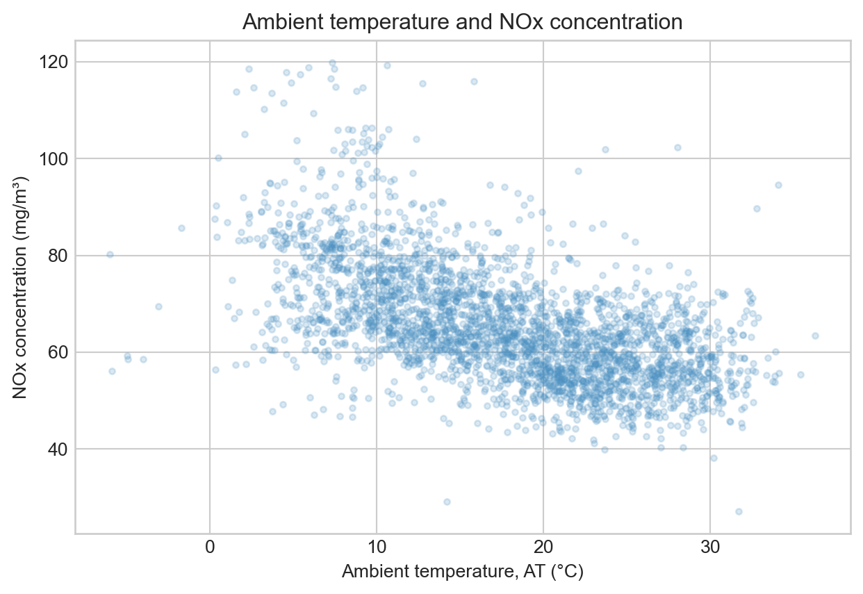
How is the NOx concentration observed at the plant associated with ambient temperature?

The goal is to build and diagnose a first regression model. It is not a complete physical model of the turbine, and it does not tell us what would happen if we intervened to change ambient temperature.

Learning objectives

Define a response, predictor, and residual.
Explain why ordinary least squares minimizes mean squared error.
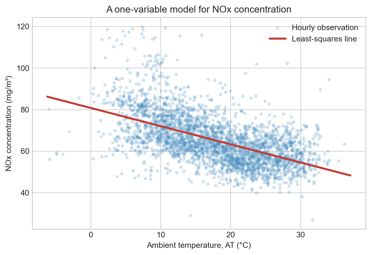
Fit and interpret a one-variable least-squares line.
Use residuals and \(R^2\) to assess in-sample fit.
Distinguish association from causation.

1. Load the course dataset

The Foundations notebooks introduced this hourly gas-turbine dataset. We repeat the setup here so the notebook runs independently in Colab. Each row is an hourly aggregate of plant measurements.

import numpy as np
import pandas as pd
import matplotlib.pyplot as plt
import statsmodels.api as sm
from pathlib import Path
from urllib.request import urlretrieve

plt.style.use("seaborn-v0_8-whitegrid")
DATA_URL = "https://raw.githubusercontent.com/changyaochen/MECE4520/master/site/data/gas-turbine-course.csv"
data_path = next((path for path in [Path("../data/gas-turbine-course.csv"), Path("site/data/gas-turbine-course.csv"), Path("gas-turbine-course.csv")] if path.exists()), Path("gas-turbine-course.csv"))
if not data_path.exists():
    urlretrieve(DATA_URL, data_path)
data = pd.read_csv(data_path)
data.head()

	campaign_year	AT	AP	AH	AFDP	GTEP	TIT	TAT	TEY	CDP	CO	NOX
0	2011	4.5878	1018.7	83.675	3.5758	23.979	1086.2	549.83	134.67	11.898	0.32663	81.952
1	2011	4.2932	1018.3	84.235	3.5709	23.951	1086.1	550.05	134.67	11.892	0.44784	82.377
2	2011	3.9045	1018.4	84.858	3.5828	23.990	1086.5	550.19	135.10	12.042	0.45144	83.776
3	2011	3.7436	1018.3	85.434	3.5808	23.911	1086.5	550.17	135.03	11.990	0.23107	82.505
4	2011	3.7516	1017.8	85.182	3.5781	23.917	1085.9	550.00	134.67	11.910	0.26747	82.028

2. Understand the measurements

Before focusing on one relationship, orient yourself to the full system.

Column	Meaning
campaign_year	Data-collection campaign year (2011–2015)
AT	Ambient temperature (°C)
AP	Ambient pressure (mbar)
AH	Ambient humidity (%)
AFDP	Air-filter differential pressure (mbar)
GTEP	Gas-turbine exhaust pressure (mbar)
TIT	Turbine inlet temperature (°C)
TAT	Turbine-after temperature (°C)
TEY	Turbine energy yield (MWh)
CDP	Compressor discharge pressure (mbar)
CO	Carbon monoxide concentration (mg/m³)
NOX	Nitrogen oxides concentration, NO + NO₂ (mg/m³)

3. Focus on ambient temperature and NOx

For this first model, use AT, ambient temperature in °C, as the predictor and NOX, NOx concentration in mg/m³, as the response.

regression_data = data[["AT", "NOX"]].dropna()
print(f"Observations used: {len(regression_data):,}")
regression_data.describe()

Observations used: 36,733

	AT	NOX
count	36733.000000	36733.000000
mean	17.712726	65.293067
std	7.447451	11.678357
min	-6.234800	25.905000
25%	11.781000	57.162000
50%	17.801000	63.849000
75%	23.665000	71.548000
max	37.103000	119.910000

4. Look before fitting

A scatterplot lets us see the relationship before asking a model to summarize it. The fitted model below will use every available observation.

plot_data = regression_data.sample(n=3_000, random_state=4520)
fig, ax = plt.subplots(figsize=(7.5, 4.8))
ax.scatter(plot_data["AT"], plot_data["NOX"], alpha=0.2, s=10, color="#4a90c2")
ax.set(xlabel="Ambient temperature, AT (°C)", ylabel="NOx concentration (mg/m³)", title="Ambient temperature and NOx concentration")
plt.show()

The cloud slopes downward, but it is far from a perfect line.

5. State the model

Treat NOx concentration as the response, \(Y\), and ambient temperature as the predictor, \(X\):

\[ Y_i = \beta_0 + \beta_1 X_i + \varepsilon_i. \]

Here, \(\varepsilon_i = y_i - \hat{y}_i\) is the residual: the vertical difference between an observation and its prediction.

6. Choose a loss function

A raw mean residual can cancel positive and negative errors. Mean absolute error (MAE) avoids cancellation, but its absolute-value kink makes optimization less convenient. Ordinary least squares uses mean squared error (MSE):

\[ \mathcal{L}_{\mathrm{MSE}}(\beta_0, \beta_1) = \frac{1}{n}\sum_{i=1}^{n}\left(y_i - \beta_0 - \beta_1x_i\right)^2. \]

Squaring prevents cancellation and gives larger errors more weight.

x = regression_data["AT"]
y = regression_data["NOX"]
candidate_lines = pd.DataFrame({"intercept": [70.0, 80.8, 90.0], "slope": [-0.50, -0.88, -1.20]}, index=["A", "B", "C"])

def residual_summaries(intercept, slope):
    residual = y - (intercept + slope * x)
    return pd.Series({"mean residual": residual.mean(), "MAE": residual.abs().mean(), "MSE": (residual**2).mean()})

loss_table = candidate_lines.apply(lambda line: residual_summaries(line["intercept"], line["slope"]), axis=1)
candidate_lines.join(loss_table)

	intercept	slope	mean residual	MAE	MSE
A	70.0	-0.50	4.149430	7.926254	118.918579
B	80.8	-0.88	0.080266	7.369149	93.897656
C	90.0	-1.20	-3.451661	8.248357	111.652396

7. Fit the least-squares line

Simple linear regression has a closed-form MSE minimizer. statsmodels performs that optimization after we add a constant column for the intercept.

X = sm.add_constant(x)
model = sm.OLS(y, X).fit()
intercept = model.params["const"]
slope = model.params["AT"]
pd.Series({"intercept (mg/m³)": intercept, "slope (mg/m³ per °C)": slope})

intercept (mg/m³)       80.796532
slope (mg/m³ per °C)    -0.875273
dtype: float64

temperature_grid = np.linspace(x.min(), x.max(), 200)
fig, ax = plt.subplots(figsize=(7.5, 4.8))
ax.scatter(plot_data["AT"], plot_data["NOX"], alpha=0.2, s=10, color="#4a90c2", label="Hourly observation")
ax.plot(temperature_grid, intercept + slope * temperature_grid, color="#c43c35", linewidth=2.5, label="Least-squares line")
ax.set(xlabel="Ambient temperature, AT (°C)", ylabel="NOx concentration (mg/m³)", title="A one-variable model for NOx concentration")
ax.legend()
plt.show()
print(f"Fitted line: NOx = {intercept:.2f} {slope:+.3f} × AT")

Fitted line: NOx = 80.80 -0.875 × AT

Interpret the slope

The fitted slope is the predicted difference in NOx concentration associated with a one-degree-Celsius difference in ambient temperature. This is an association, not an intervention claim.

8. Inspect the residuals

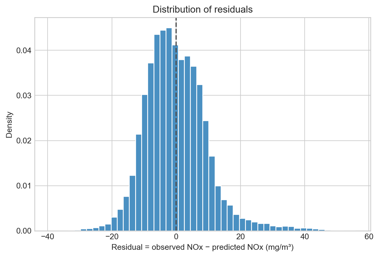
Residuals reveal the variation that the line leaves unexplained. Start with their distribution: what size error is typical, and are there unusually large errors? A residual histogram can assess whether a Normal approximation is plausible, but it cannot prove a Normal-error assumption.

residual = model.resid
residual_sd = residual.std(ddof=2)
fig, ax = plt.subplots(figsize=(7.5, 4.8))
ax.hist(residual, bins=50, density=True, color="#4a90c2", edgecolor="white")
ax.axvline(0, color="#4d4d4d", linestyle="--", linewidth=1.5)
ax.set(xlabel="Residual = observed NOx − predicted NOx (mg/m³)", ylabel="Density", title="Distribution of residuals")
plt.show()
print(f"Residual mean: {residual.mean():.3e} mg/m³")
print(f"Residual SD: {residual_sd:.2f} mg/m³")

Residual mean: -9.508e-15 mg/m³
Residual SD: 9.69 mg/m³

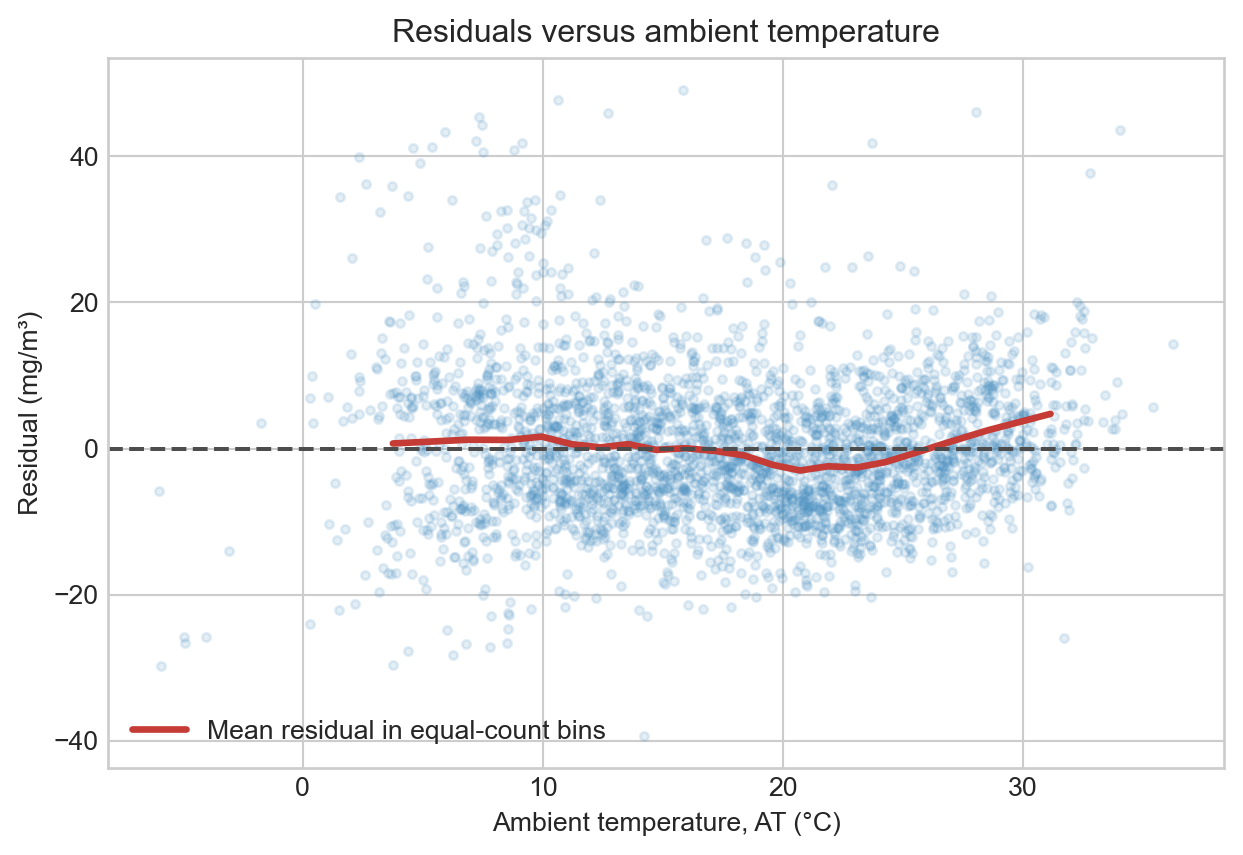
A residual mean near zero is guaranteed by OLS when the model includes an intercept. More revealing questions are whether the center stays near zero and whether the spread stays about the same width across the range of AT values.

diagnostic_data = regression_data.assign(residual=residual)
diagnostic_sample = diagnostic_data.sample(n=3_000, random_state=4520)
binned_residuals = diagnostic_data.assign(AT_bin=lambda frame: pd.qcut(frame["AT"], 20)).groupby("AT_bin", observed=True)[["AT", "residual"]].mean()

fig, ax = plt.subplots(figsize=(7.5, 4.8))
ax.scatter(diagnostic_sample["AT"], diagnostic_sample["residual"], alpha=0.15, s=10, color="#4a90c2")
ax.plot(binned_residuals["AT"], binned_residuals["residual"], color="#c43c35", linewidth=2.5, label="Mean residual in equal-count bins")
ax.axhline(0, color="#4d4d4d", linestyle="--", linewidth=1.5)
ax.set(xlabel="Ambient temperature, AT (°C)", ylabel="Residual (mg/m³)", title="Residuals versus ambient temperature")
ax.legend()
plt.show()

The red line summarizes the average residual at nearby temperature values. A pattern above and below zero suggests that a straight line misses systematic structure. A changing vertical spread suggests heteroscedasticity. These diagnostics identify useful next modeling steps, such as nonlinear features, additional predictors, or time-aware validation.

9. Summarize fit with \(R^2\)

A mean-only baseline predicts every observation with \(\bar{y}\). Its total squared error is the total sum of squares (TSS). The regression’s squared error is the residual sum of squares (RSS):

\[ R^2 = 1 - \frac{\mathrm{RSS}}{\mathrm{TSS}}. \]

Thus, \(R^2\) is the fraction of baseline squared error that the fitted line removes. It describes in-sample fit, not causality or future predictive accuracy.

mean_only_prediction = y.mean()
tss = ((y - mean_only_prediction) ** 2).sum()
rss = (residual**2).sum()
r_squared = 1 - rss / tss
pd.Series({"TSS (mean-only baseline)": tss, "RSS (regression line)": rss, "R²": r_squared})

TSS (mean-only baseline)    5.009658e+06
RSS (regression line)       3.448860e+06
R²                          3.115577e-01
dtype: float64

Check-in

Why can the raw mean residual be misleading as a loss function?
What would a residual-versus-AT plot look like if a straight-line conditional mean were adequate?
If \(R^2 \approx 0.31\), what does that say about the regression line relative to the mean-only baseline?

Keep your answers in your own notes. Later regression materials will introduce confidence intervals, hypothesis tests, additional predictors, and out-of-sample validation.

Return to the Regression page