Notes for Generative AI learning, part 1

This is my notes when reading the book “Generative Deep Learning, 2nd Edition” by David Foster, published by O’Reilly (link).

Chapter 1 and 2

Mostly introductory to generative models and neural networks. One main takeaway is that, in supervised learning (arguably the most common type of machine learning), we try to learn \(P(y | x)\), where \(y\) is the label and \(x\) is the input. In generative models, we try to learn \(P(x)\), and to sample from it to generate new data.

At times, we try to decompose \(P(x)\) into \(P(x | z)\), where \(z\) is a latent variable. This is the main idea behind Autoencoder which we will discuss in the next chapter.

Chapter 3. Variational Autoencoders (VAEs)

A simple autoencoder is a neural network that takes an input and maps it to a fixed point in the latent space (encoder), and then from this point, we try to create (that is, reconstruct) the input (i.e., an image).

How to create an image from a latent vector? With tensorflow/keras, we can use either the Conv2DTranspose layer or the UpSampling2D layer. The idea is the same: we first increase the size of the 2D space, by either filling with zeros or repeating the nearest pixel. With the enlarged 2D space, we then apply the convolutional operation with stride of 1.

The key idea of VAE is instead of mapping an input to a fixed point in the latent space, we map it to a (standard normal) distribution in the latent space.

The model parameters now will also include the parameters of the distribution in the latent space, for example, if the latent space is 100-dimensional and we want to use a normal distribution, we will have 200 parameters to learn: 2 for each dimension. Accordingly, the loss function will include both the reconstruction loss and the Kullback–Leibler (KL) divergence loss. The latter is to measure the similarity between the learned distribution and a standard normal distribution: we also want to minimize this loss. A good explanation of the intuition can be found here and the derivation between two Normal distributions can be found here.

Latent space arithmetic

A natural question is, can we find meanings of the latent space, e.g., a certain dimension (or vector) corresponds to a person of the image? It can be done, with the help of labels: if we can label all the images with a person it it, and all the images without any person, we can then calculate the difference of the the average latent vector of the two groups, and the resulting vector can be interpreted as the “person” vector.

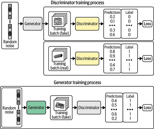
Chapter 4, Generative Adversarial Networks

When training the generator, why do we set the label as “1”, as if the generated image is real? Note that in this phase, we assume we have a perfect discriminator which outputs the probability of the image being real. Among the images generated by the generator, if by chance we create a truly real image, this will be correctly identified by the discriminator as real (giving a high probability), therefore, we want to reward such a situation by setting the label as “1” and use the binary cross-entropy as the loss function.

At the end of the day, we want the generator to generate images that are indistinguishable from the real images.

Training of a GAN

Wasserstein GAN

The original GAN has a few issues, e.g., mode collapse, and the training is not stable. Wasserstein GAN (WGAN) solves these issues by using the Wasserstein distance as the loss function. In the original GAN, the loss function is the binary cross-entropy, for both the discriminator and the generator. In WGAN, the output (prediction), \(p_i\) for the discriminator is not a probability, but a real number, ranging from negative infinity to positive infinity. As such, the discriminator is now also called the critic. The labels, \(y_i\), also change from 0 and 1 to -1 and 1. After this modification, the (Wasserstein) loss function is defined as

\[-\frac{1}{n} \sum_{i=1}^{n} y_i p_i,\]

where \(n\) is the number of samples.

There are few other tricks in WGAN to stabilize the training, e.g., weight clipping, gradient penalty (GP, making it WGAN-GP), etc. To summarize:

• There is no sigmoid activation in the final layer of the critic.
• The WGAN-GP is trained using labels of 1 for real and –1 for fake.
• A WGAN-GP uses the Wasserstein loss.
• Include a gradient penalty term in the loss function for the critic.
• Train the critic multiple times for each update of the generator.
• There are no batch normalization layers in the critic.

Conditional GAN (CGAN)

In the case of VAE, we can find a way to find meanings in the latent space, such as “smiling”, by labeling the corresponding images. More importantly, we can ask the model to generate the desired outcome, by providing the corresponding latent vector. Namely, we have learned \(P(x | z)\), and then we can provide \(z\) to generate the corresponding \(x\).

In the vanilla GAN, we cannot do this, as the input to the generator is a random noise. What we have achieved, is to learn \(P(x)\), and to sample from it. We have little control of the outcome, say, to generate an image with a car.

In the case of GAN, we can still fix this by giving the image labels, and modify the architecture of the GAN with an additional input (to both critic/discriminator and generator) to reflect this information. This is called a conditional GAN (CGAN).

In terms of training, CGAN is similar to GAN, only needing to modify the dimension to accommodate the additional dimensions.