Notes for Generative AI learning, part 2

Chapter 5. Autoregressive Models

An autoregressive model takes the preceding elements of a sequence as input to predict the next element. For example, a time-series model to predict the stock price for next day. In the context of generative model, a typical application of autoregressive model is in the generation of text, where the model predicts the next word in a sentence given the preceding words.

Recurrent Neural Network (RNN)

RNN (Recurrent Neural Network) is a type of autoregressive model, that predicts the next element in a sequence. The elements of the sequence (e.g., words from a vocabulary, say, English) are usually represented as embeddings (a vector of real numbers), that is, a one-to-one mapping such as "word" -> [0.1, 0.2, 0.3, ...] (the key of the mapping is usually an integer, acting as the index of the word in the vocabulary).

The characteristics of a RNN layer is the “hidden state”, which carries a recurrent nature. As the image below shows, to get a prediction from the RNN layer, one needs to feed it with the sequence of \([x_1, x_2, x_3, ...]\) one by one, in order to get \(x_t\) (a.k.a, \(y\)). In this process, the hidden state \(h_{i-1}\) from the previous step \(i\) is combined with the input \(x_i\), to create, among other things, the new hidden state \(h_i\). This new hidden state will be used for the next iteration.

How does a RNN layer work. The input sequence is 200-long, and each element is a 100-dimensional vector (embedding). The hidden state is 158-dimensional. The input element is encoded as a 100-dimensional vector. The hidden state is represented as a 158-dimensional vector.

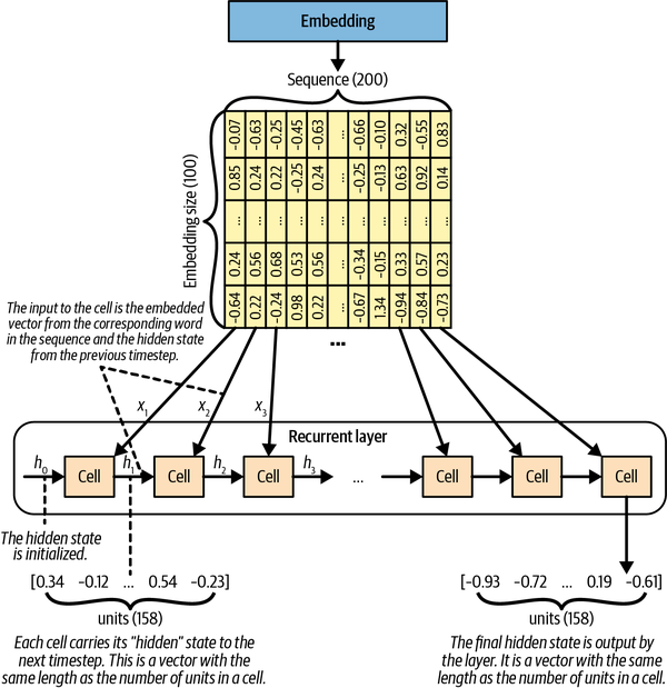
Given the output of the RNN layer, how can we produce the desired output, which is an element (e.g., an English word) from the vocabulary? The answer is to use a dense layer, whose output size equals to the size of the vocabulary. The dense layer will take the output of the RNN layer, and take the softmax activation to produce the probability distribution whose support is the vocabulary. We can then sample from this distribution to get the next word.

When training the RNN model, the loss function is usually the categorical cross-entropy loss, which measures the difference between the predicted probability distribution and the true distribution. Here the support of the distribution is the vocabulary.

LSTM (Long Short-Term Memory)

The recurrent nature of RNN is designed for it to “remember” information from previous elements. However, it is not very good at remembering information from very far back: a naive approach would be including a longer sequence of elements during the training process. In practice, this leads to the vanishing/exploding gradient problem, where the network is incapable to learn from the long-term dependencies.

The LSTM (Long Short-Term Memory) is a type of RNN that is designed to address this issue. It modifies the RNN layer by adding a few “gates”, each of which is responsible for a dedicated task. For example, the “forget gate” is responsible for deciding whether to forget (i.e., not to remember) information from the previous elements, and the “input gate” is responsible for deciding how much information to keep (i.e., not to forget) from the current element.

The figure below shows the schematic of the LSTM cell (copied from Chris Olah’s blog): aside from the hidden state \(h\), the LSTM cell also keeps (outputs) a cell state \(C\) (the upper brach that flows through the cell). The values of both the hidden state and the cell state are updated via a series of matrix multiplications and activation (with either sigmoid, \(\sigma\), or hyperbolic tangent, \(\tanh\)).

A concise schematic of the LSTM cell. The upper branch represents the cell state, and the lower branch represents the hidden state.

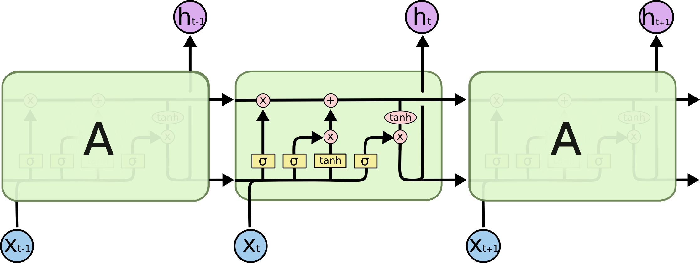
A naive question (at least for me) is: why do we need both sigmoid and \(\tanh\) activation, mathematically, they can be combined with just one \(\tanh\) function. The answer stems from that, by separating the two activation functions, the LSTM cell can learn more efficiently, as the two functions are responsible for different tasks.

Gated Recurrent Unit (GRU)

The LSTM introduces a cell state to keep track of the long-term dependencies, which inevitably increases the complexity of the model. The GRU (Gated Recurrent Unit) is a simplified version in that it maintains just the hidden state, but makes effort how the hidden state is updated, by taking a page from LSTM. For example, it combines the forget and input gates into a single “update gate”.

PixelCNN: combining space and time

Previously, we have learned that we can use CNN (Convolutional Neural Network) to incorporate the spatial information of the input data (e.g., images) to learn the underlying patterns.

There isn’t an apparent sequential nature with regard to the pixels in an image, however, one could argue that, if we know enough “leading” pixels, we can predict what the next pixel should be. Here we can define the ordering of the pixels from top-left to bottom-right, row by row.

This is the intuition behind PixelCNN, which combines the sequential nature of the autoregressive model to the spatial nature of CNN. The structure of PixelCNN is quite similar to a CNN based autoencoder, only that we introduce a special “masked” convolutional layer, where:

• The “second half” of the convolutional kernel is masked out, so that the convolutional layer can only “see” the pixels that have been processed.
• The center pixel of the kernel is either masked out, or not.

At generation time, we can feed the model with a partially filled image (or a blank image), and let the model predict the next pixel, based on the preceding pixels, so on and so forth, until the image is fully generated.

I personally find the PixelCNN model a bit less practically useful, as it doesn’t allow the user to provide meaningful input to the model, such as a text prompt, or a latent vector (maybe not so meaningful…). However, it is a good example to show how one can combine different types of neural networks, in this case, spatial and sequential, to learn the underlying patterns of the data.

Again, like the vanilla GAN, the PixelCNN learns \(P(x)\), instead of \(P(x|z)\).

Chapter 6. Normalizing Flow Models

The central idea for a generative model is to learn the underlying distribution \(P(x)\) of the data, so that we can generate new data by sampling from it. However, \(P(x)\) is usually complex, and we usually resort to a “simpler” distribution, as in the case of VAE, the distribution of the latent variable \(P(z | x)\).

The idea of normalizing flow models is similar, but we want to learn the distribution of the latent variable $$P(z) directly. Also, we want to impose some constraints on the functional form of this “base” distribution, e.g., as a Normal distribution.

Change of variables in the normalizing flow model. Here the data is denoted as \(y\), instead of the usual \(x\). Reference.

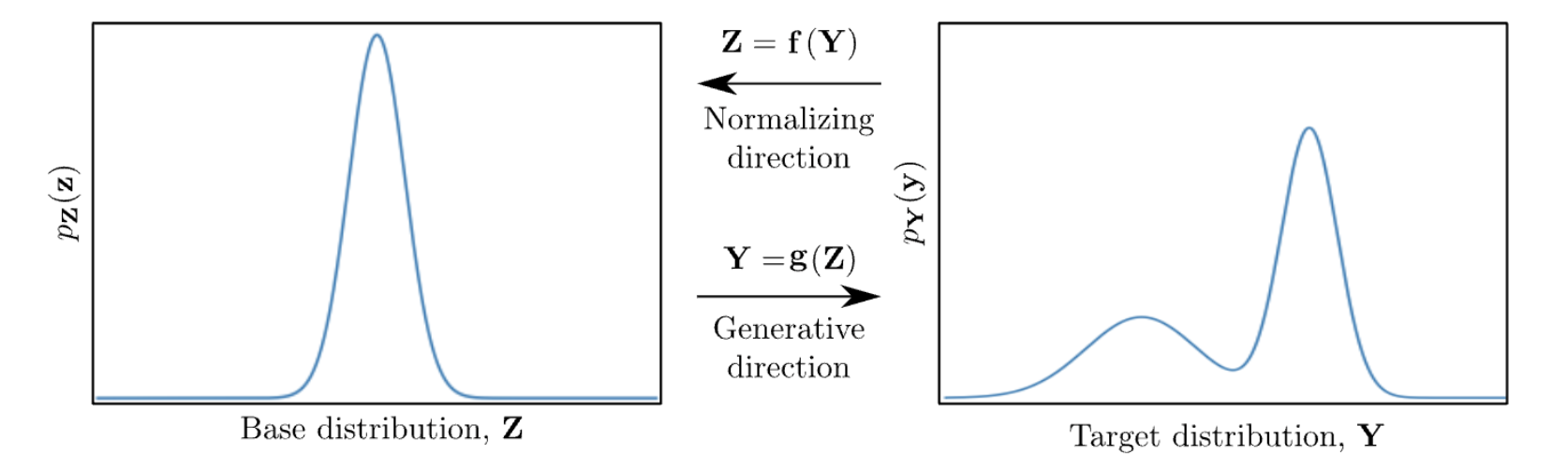
This technique, known as “change of variables”, is common in probability theory. The function \(f\) can be viewed as the encoder in the VAE model, mapping data (\(x\) or \(y\)) to the latent variable \(z\), and the function \(g\) can be viewed as the decoder, mapping \(z\) back to the data space. However, unlike VAE where the encoder and decoder are learned independently, here \(f\) is the inverse of \(g\). Therefore, once \(g\) is learned, \(f\) is also set. Such a pair of functions is called “bijection”, or bijective function.

In the context of generative models, the function \(g\) (a generator) “pushes forward” the base density \(P(z)\) (sometimes referred to as the “noise”) to a more complex density. This movement from base density to final complicated density is the generative direction.

The inverse function \(f\) moves (or “flows”) in the opposite, normalizing direction: from a complicated and irregular data distribution towards the simpler, more regular or “normal” form, of the base measure \(P(z)\). This view is what gives rise to the name “normalizing flows” as \(f\) is “normalizing” the data distribution. This term is doubly accurate if the base measure \(P(z)\) is chosen as a Normal distribution as it often is in practice.

Coupling flows

We still need to learn the function (i.e., mapping, transformation) \(f\), which is usually done by a neural network. There are different families of functions that can be used to model \(f\), for example, a simple linear transformation of \(x\). In this book, the authors focus on the “coupling flows”, which is a type of function that splits the input to two parts, and the mapping (transformation) is done by applying a function to one part, and conditioning on the other part. For example, if the input \(x\) has 4 dimensions, we can split it to two parts, the first two dimensions \([x_1, x_2]\) and the rest, \([x_3, x_4]\). The transformation can then be:

\[\begin{align*} [y_1, y_2] &= [x_1, x_2] \odot \exp(s([x_3, x_4])) + t([x_3, x_4]),\\ [y_3, y_4] &= [x_3, x_4], \end{align*}\]

where \(\odot\) is the element-wise multiplication, and \(s\) and \(t\) are the scaling and translation functions, respectively. In practice, we can pass data with all the 4 dimensions to both of above operations, but setting the unwanted dimensions to zero, e.g., \(x_3\) and \(x_4\) in the first operation.

In this way, we ensure:

• The inverse transformation (from \(y\) to \(x\)) is well-defined.
• The Jacobian of the transformation is easy to compute. The Jacobian is required to compute the probability density of the transformed data, and an efficiently computed Jacobian is crucial for the training process.

Now we have described how one step of coupling flow works. In practice, we can stack multiple coupling layers, and importantly, alternating the split, that is, which part of the input is transformed and which part is kept unchanged. This is the basic of the “realNVP” (Real-valued Non-Volume Preserving) model.

When training the realNVP model, we want to learn the scaling and translation functions \(s\) and \(t\) for each coupling layer, while the loss function is the negative log-likelihood, taken with respect to the target distribution \(P(x)\).

Although we do not know the target distribution \(P(x)\), however, the negative log-likelihood can be computed by the change of variables formula, given the base distribution \(P(z)\), the transformation (\(s\)s and \(t\)s), and the Jacobian of the transformation.