Notes for Generative AI learning, part 3

I am having a hard time grasping the energy-based model and the related diffusion models, therefore I will skip this part for now.

Chapter 9: Transformers

The most important architecture in the recent years is without a doubt the transformer. It originates in the Natural Language Processing (NLP) field, and has been applied to other fields, notably, in modeling sequential events. This includes autoregressive models (predicts the next token in a sequence, think chatGPT), and also sequence-to-sequence models (translation between languages).

The vanilla transformer (namely, the original 2017 paper) discusses an autoregressive fashion. The improvement of the transformer over the previous state-of-the-art (Recurrent Neural Networks, RNNs) is the ability to parallelize the computation. In RNN, each token in the sequence is processed sequentially, and the latent information from the last token in the sequence is used for inference (e.g., predict the next token). This requires all the relevant information to be encoded the last hidden state, therefore greatly limits how well a RNN can “pay attention” to the information from the earlier portion of the sequence.

Basic transformer mechanism

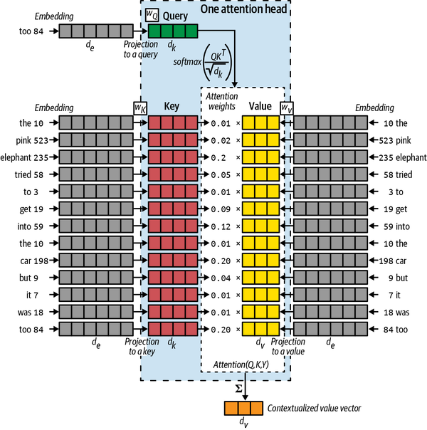
The transformer architecture essentially exposes all the hidden states from all the tokens in the sequence at once. To do so, it sets up a mechanism, such that for different tasks (“query”), to “pay attention” to different previous tokens (“key”) with different degrees of relevance (“value”).

Take the following example: we want to predict the next word after “the pink elephant tries to get into the car but it was too __”. We, as human, would think a proper word for the blank is “big”, not because we have seen “pink” in the sentence, but because we have seen “elephant” and “car” in the sentence (plus our knowledge of the world). Under the transformer setting, the query is the word “too” (as we are asking for the next word after it), and the keys are all the words in the sentence. We want to find the “relevance” between the query and the keys, and in mathematical terms, we can express them as the product between the query vector and the key vectors (_i.e., a matrix). The resulting vector prescribes how much attention (i.e., weight) the query should pay to each key.

We can then apply these weights to the values, usually after normalizing the weights (e.g., softmax). The value for each key can be thought as the unweighted contribution. By multiplying the attention weights to the values, we get the so-called contextualized value (vector), which is used to make the prediction.

How does the query, key, and value work in the attention head. Note that the dimensions for the key and the value does not have to be the same, but the query and the key must have the same dimension.

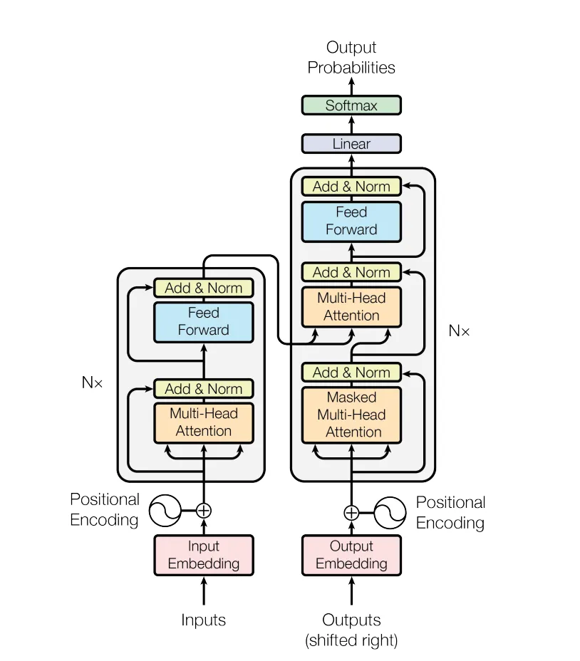
What described above constitutes a single attention head. The transformer architecture consists of multiple attention heads, and the output from each attention head is then concatenated and passed through a few other layers, such as residual connection, layer normalization, and fully connected layers. These components have less to do with the attention mechanism, but mostly needed to the neural network to train.

The query-key-value configuration allows us to pay attention to multiple tokens at once, however, it only takes one query (vector) at a time. We can further speed up t by taking multiple queries (a query matrix, so to speak). One caveat is that we need to apply an additional diagonal “mask” matrix (causal mask), to avoid data leakage.

Positional encoding

The transformer architecture speeds up the training by looking at the previous tokens “at the same time”, however, this also imposes an issue as the ordering information is lost. For example, the following two sentences have the same tokens but we likely will make different predictions.

The dog looked at the boy and …​ (barked?)

The boy looked at the dog and …​ (smiled?)

To solve this issue, one need to feed the position information of each token. The original paper uses a trigonometric function, but one can use a more general embedding layer, additive to the token embedding, to encode the position.

Extensions of transformers

The transformer model, at the end of the day, tries to learn a good representation (embedding) of each token, but we have different ways to use this representation.

With the popularity of ChatGPT, we are more familiar with the “decoder-only” type model. In this case, we simply predict the next token, and next, and next…, basically, to complete the sentences. It is worth noting that, the input tokens to a “decoder-only” model are encoded (mapped to embeddings), however, it is called decoder-only is because there isn’t a transformer based encoder block in the model architecture, but rather just a decoder block(s).

Example(s): GPT.

Similarly, an “encoder-only” model has only the encoder block. They are not used for auto-regressive type of problems, but rather for tasks such as classification (e.g., named entity recognition, NER). In this case, we do not need to apply the causal mask, as the encoders are allowed to learn everything about the sequence (bi-directional).

Example(s): Bidirectional Encoder Representations from Transformers, BERT.

For completeness, there is also “encoder-decoder” model, that kind of combines the properties of the two aforementioned types. Such a model can first understand the input sequence “deeply”, then produce the output in an auto-regressive manner. Machine translation, summarization are the most suited application areas.

Example(s): Text-to-Text Transfer Transformer, T5. Bidirectional and Auto-Regressive Transformers, BART.