How to sample from a distribution

We have come accustom to the ease of generating samples from a given distribution, but I become curious about how actually it is done. In this post, I will describe 4 sampling methods. They are not necessarily the most advanced techniques, but it will get the job done. This is largely based on the materials from here.

Preliminary: uniform random number generator

We need some randomness to generate samples, and we can seed all the randomness from a uniform random number generator, which gives us a random number between 0 and 1 with equal probability. This can be done using simple arithmetic such as

\[x_{i + 1} = (a \cdot x_i + c) \mod m,\]

where \(a\), \(b\), and \(m\) are predefined constants. This operation will give us a sequence of numbers, and with different initial values of \(x_0\), we can get different sequences. To convert the value to between 0 and 1, we can simply divide the number by \(m\).

This approach has the desired properties of deterministic randomness, as with the same initial value of \(x_0\) (seed), we will get the same sequence of numbers.

The choices of \(a\), \(b\), and \(m\) are important, as they determine how apparent the randomness is. In practice, we set \(m = 2^{b}\) where \(b\) is the number of bits in a binary computer word. \(a\) should be chosen such that it is equal to 1 in modulo 4 arithmetic (i.e., 1, 5, 9, 13 …. ) and that \(c\) should be an odd number.

Now we have a uniform random number generator, so that we can easily draw samples \(R \sim U(0, 1)\).

Inversion method

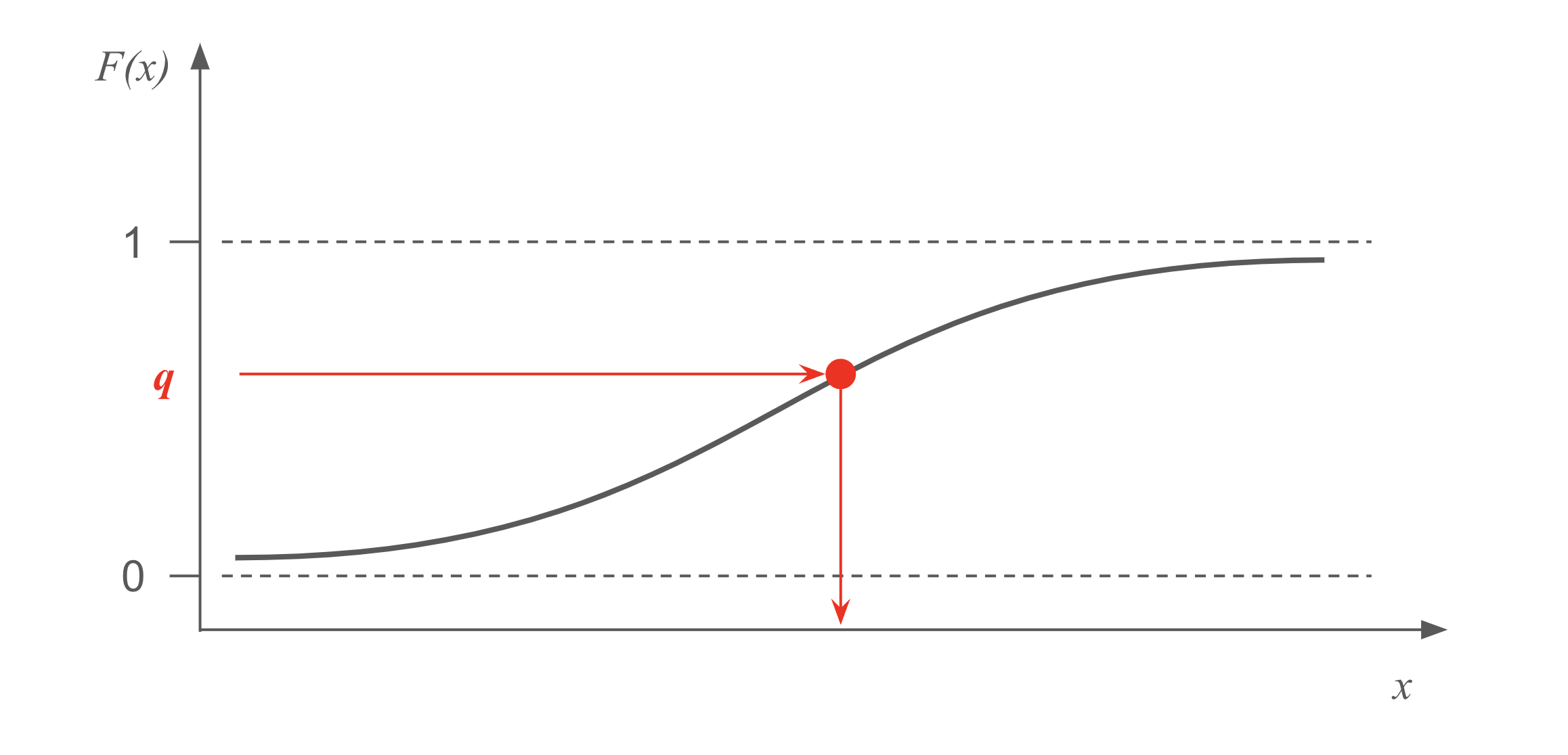
To sample from a distribution, we often time have the probability density function (pdf), \(f(x)\), or probability mass function (pmf) in the discrete case. There are situations where we can integrate the pdf to obtain the cumulative distribution function (CDF), \(F(x)\), and if we are still lucky, we can invert the CDF as, \(F^{-1}(q)\).

With \(F^{-1}(q)\) in hand, we can sample from \(f(x)\) by first drawing \(u\) from \(U(0, 1)\), and then setting \(x = F^{-1}(u)\). The logic is quite straightforward: we map from the vertical axis of the CDF (quantile), to the horizontal axis of the pdf (value). Since the quantile if uniformly random, we achieve the goal of random sampling from the given distribution.

How we map a uniform random number to a sample from a distribution using the inversion method.

Below are examples of pdf, CDF, and inverse CDF for some common distributions. Note that only the first two distributions have closed-form inverse CDFs, hence applicable to the inversion method.

Distribution	pdf, \(f(x)\)	CDF, \(F(x)\)	Inverse CDF, \(F^{-1}(q)\)
Exponential	\(\lambda e^{-\lambda x}, \, x \geq 0\)	\(1 - e^{-\lambda x}, \, x \geq 0\)	\(-\frac{1}{\lambda} \ln(1 - q)\)
Logistic	\(\frac{e^{-(x-\mu)/s}}{s(1+e^{-(x-\mu)/s})^2}\)	\(\frac{1}{1 + e^{-(x-\mu)/s}}\)	\(\mu + s \ln \left( \frac{q}{1 - q} \right)\)
Normal	\(\frac{1}{\sqrt{2\pi}\sigma} e^{-\frac{(x - \mu)^2}{2\sigma^2}}\)	\(\frac{1}{2} \left[ 1 + \text{erf} \left( \frac{x - \mu}{\sigma \sqrt{2}} \right) \right]\)	No closed form
Beta (\(\alpha, \beta\))	\(\frac{x^{\alpha-1}(1-x)^{\beta-1}}{B(\alpha, \beta)}\)	\(I_x(\alpha, \beta)\)	No closed form
Gamma (\(k, \theta\))	\(\frac{1}{\Gamma(k)\theta^k} x^{k-1} e^{-x/\theta}\)	\(P(k, x/\theta)\)	No closed form

We can see that for normal, Beta, and Gamma distributions, we can not use inversion methods, but we will explore different approaches later.

Relationships method

For distributions without closed form inverse CDFs, sometimes we can leverage its relationship to other, easily sample-able distribution (e.g., with inversion method), to generate samples.

For example, the interval between two consecutive Poisson point process follows an Exponential distribution, therefore, we can use multiple samples drawn from an Exponential distribution to generate samples from a Poisson distribution.

Similarly, we can use \(n\) samples drawn from a Bernoulli distribution to create a sample from a Binomial distribution. We can also draw \(k\) samples from an exponential distribution with mean \(\theta\) to create a sample from a Gamma distribution.

Approximation method

If the relationship method is not applicable, one can resort to approximating the distribution of interest, from other distributions that are easily sample-able. The prime example is the Normal distribution, where we can use the central limit theorem (CLT) to approximate. Essentially, we start by drawing samples from another distribution.

For example, we can take the Uniform distribution \(U(0, 1)\), then take the sample mean, \(z = (u_1 + u_2 + u_3 ... + u_k) / k\). Since we know the mean of the Uniform distribution is \(1/2\), and the variance is \(1/12\), then with large enough \(k\), we have \(\frac{z - 1/2}{\sqrt{1 / (12 \cdot k) }} \sim N(0, 1)\). From here, we can easily generate \(N(\mu, \sigma^2)\) by scaling and shifting.

A side note: for Normal distribution, we can use a more efficient, Box-Muller transform method.

Rejection method

This is the most generic method, as long as we have the pdf of the target distribution, \(f(x)\), available to us. Let’s use a contrived example to demonstrate how it works.

Let’s assume the support for the target distribution’s support is between \((a, b)\), and the maximum of the pdf is less than \(c\). We can then draw a rectangular box of height \(c\) and width \((b - a)\), and then draw a point uniformly randomly from this box. If this point is above the pdf \(f(x)\), we reject this point and draw another one. If it is below \(f(x)\), we accept this point, and treat the \(x\) value as a sample from the target distribution.

A contrived example of the rejection method. The point \((x_1, y_1)\) is rejected, whereas the point \((x_0, y_0)\) is accepted, and \(x_0\) is treated as a sample from \(f(x)\).

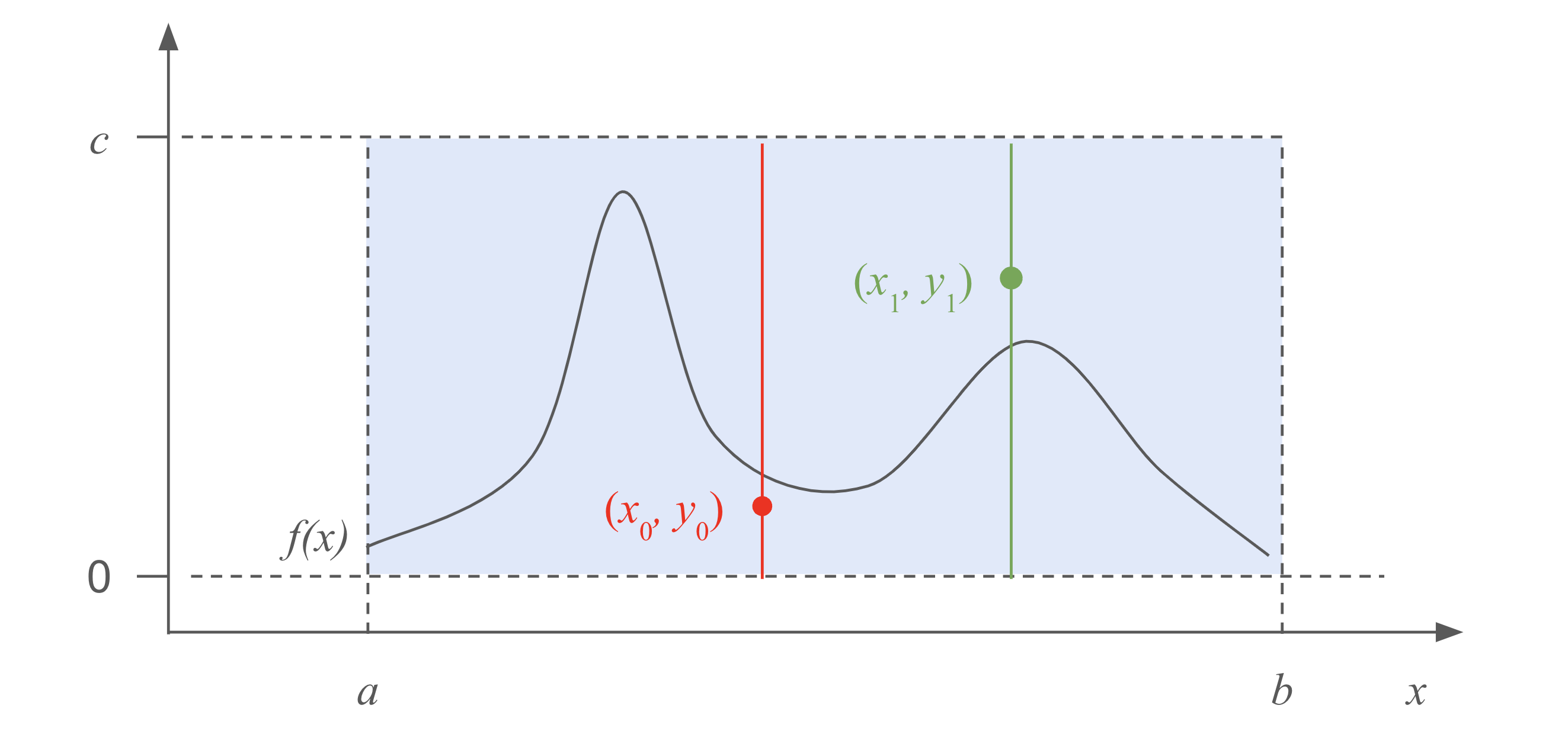
Why does this work? One can either try to understand from the geometry of the process, and think about the acceptance probability:

\[P(\text{accept} | x_0 < x < x_0 + \text{d}x) = \frac{f(x) \text{d}x}{c \text{d}x} = \frac{f(x)}{c},\]

which is proportional to \(f(x)\) up to the constant \(c\).

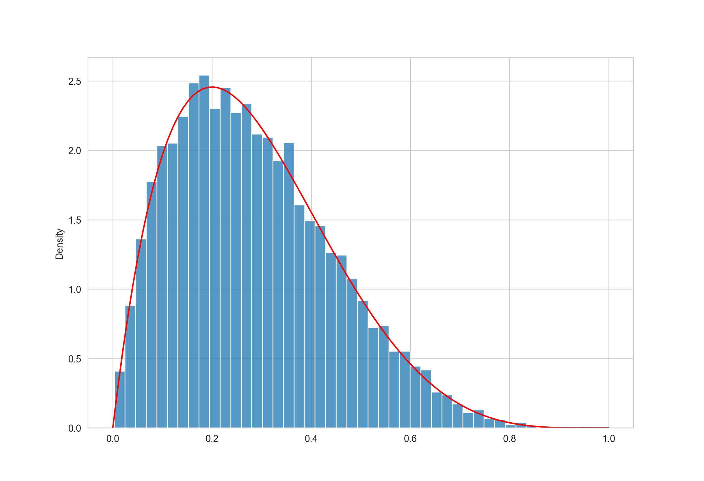
Let’s use this method to sample from a Beta distribution, whose support is conveniently defined between 0 and 1.

import numpy as np
from scipy.stats import beta

# Parameters for the Beta distribution
a, b = 2, 5  # shape parameters, whose pdf is less than 3

c = 3
N = 10_000  # number of samples

samples = []
for _ in range(N):
    accept = False
    while not accept:
        x, y = np.random.uniform(), np.random.uniform(low=0, high=c)
        if y < beta.pdf(x, a, b):  # accept
            accept = True
            samples.append(x)

When we plot the sampled values, we can see that it closely resembles the desired pdf.

Samples from a Beta distribution using the rejection method. The red line is the pdf of the Beta distribution.

Here we draw the candidate \(x\) from a Uniform distribution, and this is called the proposal distribution. We can also use other distributions as long as they are easy to sample from.

The rejection method is the most generic method, however, it does have some constraints, at least for the vanilla version discussed here. For example, the pdf of the proposal distribution must “contain” the pdf of the target distribution, and in practice, we can multiply a large constant to the proposal distribution to ensure this.

Another drawback of the rejection method is that it can be inefficient, as we might reject multiple samples before accepting one.

Conclusion

Here we showed how to sample from almost any distribution, as long as we know its pdf. Obviously there are more advanced approaches, some don’t even require the pdf to be normalized, e.g., MCMC method. But the basic idea should be similar to what we discussed here.