LIME, anyone?

For the most part of the day, we build models (at least we wish), using more and more sophisticated algorithms, achieving better and better metrics. However, the real value of any model is for it to be applied in practical settings, to deliver business values. This step can not be done with the buy-in from other stakeholders in the organization, where the ability to explain your kick-ass model is of paramount importance. At a more fundamental level, to understand why the model makes a certain prediction is equally critical for our Data Scientists as well.

However, this is not an easy task, due to the interpretability-accuracy trade-off. Take classification as an example: it is often observed that, the higher the accuracy of a model (insert random forest, neural network, etc.) achieves, the less interpretable it becomes. Errr… I feed the data to the neural network, (and after travelling through some neurons on some layers), the result just splits out. How about let’s just treat it as a black-box, and look how accurate it is on the training / validation / test sets!

This is apparently not satisfying: if the model’s performance starts to deteriorate and make wrong predictions, we don’t know what is acting up. At the very least, for that black-box, we want to know, if one perturbs the input just a little bit, how much the output will change as a result. This is a good start point to understand the black-box. An analogy is taking the numerical derivative to approximate the true derivative of a given function, in the case when obtaining the analytical derivative is not possible. By doing so for all the inputs (features) one-by-one, one can then build up some idea of how the model behaves in the vicinity of the original input.

Enters LIME, Local Interpretable Model-agnostic Explanations. LIME takes the intuition that we just built, and abstracts it in a quantitative way. The idea is rather simple: given a black-box model, \(f\), a query point, \(q\), and the result, \(f(q)\) after running \(q\) through the model, let’s randomly sample some points, \(X\), in the neighborhood of \(q\). Run these points through the model as well, to get their results, \(f(X)\). Then we will build a simple, interpretable model (e.g., logistic regression, decision tree), to map \(X\) to \(f(X)\), and this simple model will help us to explain why the black-box model returns \(f(q)\) in the first place.

As always, the devil is in the detail. The LIME authors applied some additional steps, in order to make this technique can be applied beyond simple numerical space, such as in the contexts of text and image classification. First, the original domain space is mapped to a binary vector space, \(x’\). The interpretable models are actually built in the \(x’\)-space, and later mapped back to the original domain. Second, even with an interpretable model (e.g., logistic regression), the authors define certain quantities for the interpretability, and include it as part of the objective function (see equation 1 in the paper). Third, certain distance metric is used to weight the influence for each sample point in \(X\) to \(q\). The tutorials provided by LIME are filled with excellent examples, as well as LIME’s documentation.

Nothing works better than a simple example for my own curiosity. The figure below shows a 2-dimensional classification problem with a rather random decision boundary (positive and negative areas are shown in blue and red, respectively).

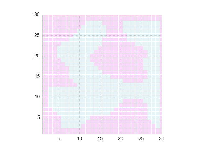
Apparently, a linear model won’t perform well in this case, as you can see here. In contrast, a nonlinear model such as Random Forest can lead to excellent metrics. The superiority of the nonlinear (i.e., black-box) model is more obvious when one tries to make predictions: say we want to predict the class of the query point (15, 15), the linear model will return the wrong answer (negative) whereas the nonlinear model returns the correct one (positive).

The natural question is, how does the nonlinear model arrive at this prediction? Here we invoke the procedure of LIME: given the query point (green hexagon in the figure below), we randomly pick some sample points around it (200 points in this case), and pass those points through the trained Random Forest model, to obtain the corresponding prediction (shown as plus and minus signs). Moreover, we also calculate the distances between those 200 points to the query point (Euclidean distance in this case): the further the sample point to the query point, the lower the weight this sample point will have. In the figure below, the size of the plus and minus signs of each sample point is proportional to its weight.

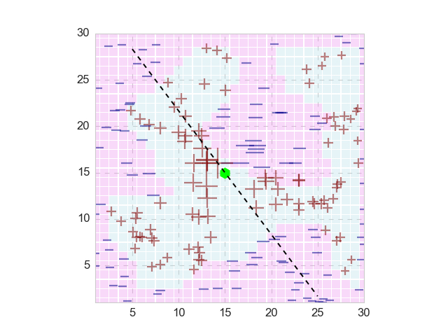
Now we are ready to build a simple, interpretable model. Note that here the 200 sample points should not be represented in the original domain space, but their transformed binary vector space. Here I train a logistic regression model, and its decision boundary that passes the original query point is shown as the black dashed line in the figure above. Surely enough, this boundary conforms the true decision boundary quite well. The coefficients of the fitted logistic regression will guide us to explain why the nonlinear model make its prediction with query point.

Here is where the LIME package shines: the inner working of LIME package will provide you the local explanation, in a rather straightforward manner. In a more realistic case, the LIME can help the user to understand why a specific prediction is made, locally. It is extremely helpful that the authors provide such an easy-to-use package, so users like me can quickly pick up and start applying to my models. LIME is also implemented in other environments such as h2o, in a slightly different format (k-LIME). It shows that the consensus about the importance of the interpretability, even this is not a new topic, but it looms even larger with the recent rapid advances in machine learning.