Notes on Reinforcement Learning: Planning

In the previous posts of this series, we have discussed how the agent can learn what is the best action to take in a given state (i.e., the policy), by interacting with the environment without a model, i.e., in the model-free setting. These approaches include Monte Carlo method, and Temporal Difference (TD) method, e.g., Q-learning. Since we do not have the complete description of the model, to apply techniques such as Dynamic Programming, we resort to the sampling from the environment, and used the past experience as the proxy to the model. Can we “squeeze more juice” from these past interactions, and treat them as if we have a model?

Combining Model-Free and Model-Based Methods

Yes, we can. In fact, this is a very common approach in practice. The idea is to use the model-free method to interact with the environment (sampling) in order to learn the underlying model, and use the model-based method to improve the policy (e.g., calculate the state-action value functions). The latter is known as the (state-space) planning.

Dyna-Q

It is not hard to see how one can intermix the sampling (or acting) and planning. For example, we can sample from the environment for one step, then update the state-action value function (via either SARSA or Q-learning). Since we just learned something from the environment, we should update our understanding of the environment, i.e., the model. This can be done simply by updating tabular information of the next state and reward. With such a table that keeps track of all the \((S, A)\) we have visited and the outcome (next state and the reward), we can run some simulation, as if this tabular model is the environment, and let the agent interact with it to keep updating the state-action value function.

Below is the pseudo-code for Dyna-Q, which is a combination of Q-learning and planning.

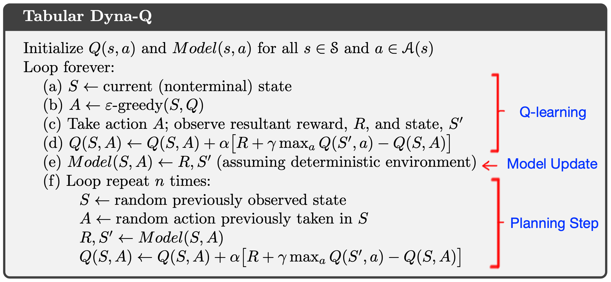
As you can see, it is largely identical to the Q-learning algorithm, except that we add a model update step (e), and a planning step (f) in which the agent interacts with the model to continue updating the state-action value function.

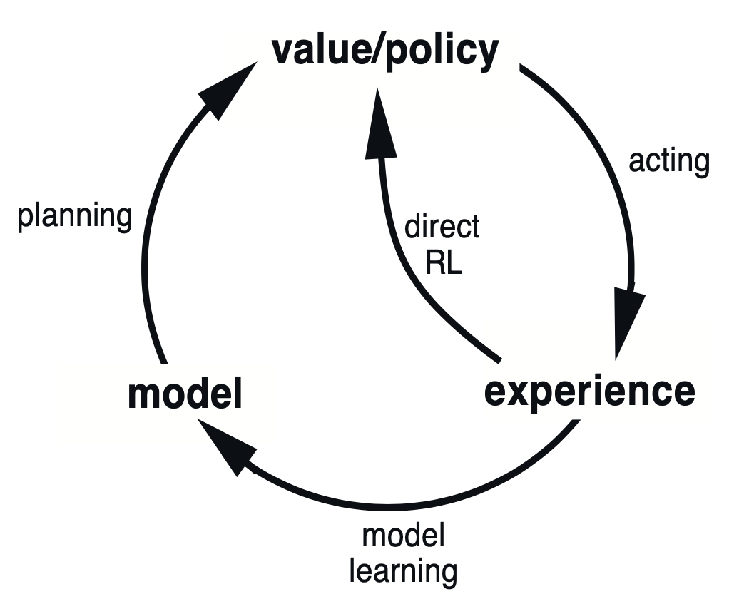
It is worth noting that, in planning, the interaction with the environment (acting) serves two purposes: 1. To update the value estimation (e.g. \(Q(S, A)\)) incrementally; 2. To update the model, which can also update the same value estimation via planning. The former is called direct RL, and the latter is called model learning.

Planning smarter

In the Dyna-Q algorithm shown above, each of the planning step starts with a random state, and apply the same state-action value function udpate rule. There can be a few issues with that.

First, the uniformly random state may not be the most efficient way to plan: after all, we would like to see changes in \(Q(S, A)\), therefore, we would like to focus on states whose q-values are recently changed, and sample the state-action pairs that leading to them. To achieve this, we can use a priority queue to keep track of the states that we have visited, and the priority is the magnitude of the change in \(Q(S, A)\). We can then sample from this priority queue to in our planning step. This is known as the Prioritized Sweeping algorithm.

Second, there is only one (or a few) acting step (sampling from the real environment) between the (possibly many) planning steps. During each planning step, we run many simulations in which we are disconnected from the real environment and solely rely on the assumption the model is correct. However, the environment might have changed, hence, we need to encourage the agent to visit outdated states (states that we have not visited for a long time) more often (the Dyna-Q+ algorithm).

Putting things together

So far, as in the first part of the Sutton and Barto, we only discussed the tabular setting, whereas the state and action spaces are discrete. However, it lays the foundation of the reinforcement learning, even for the future continuous setting. Before we proceed, let’s summarize the 3 key ideas.

Value functions

One can argue that at the heart of RL, we want to estimate some value functions, be it state, or state-action.

Backup

All the methods, e.g., value functions estimations, operate by backing up values along actual or possible state trajectories. This is of Dynamic Programming, and in the RL setting, manifests itself through the Bellman equation explicitly.

Generalized policy iteration (GPI)

Estimating the value functions is only part of the story, we still need a policy to operationalize the value functions. However, with different policies, the value functions will change. We maintain an approximate value function and an approximate policy, and they continually try to improve each on the basis of the other.

On to next

Here comes the world of infinite state and action spaces!