Normal mode

We are all quite familiar with a simple harmonic oscillator, such as a frictionless pendulum, or a mass-on-a-spring system. Since there is no friction (or energy dissipation), given a non-zero initial condition, it will swing back-and-forth, with the same amplitude, and the same frequency. Mathematically speaking, its dynamic can be described with a simple second order Ordinary Differential Equation (ODE), \(\ddot{x} + \omega^2 x = 0\), where \(\omega\) is the resonant frequency. For the sake of simplicity, I will let \(\omega\) = 1. Apparently, \(x = A \sin{\omega t}\) is a solution, and the value \(A\) is determined by the initial conditions.

However, things will be different there is another oscillator coming into play, and the second oscillator interacts with the first one. Below is a schematic picture of such condition (courtesy of wikipedia).

Let’s call the motion of the left oscillator \(x_1\), and that of the right oscillator \(x_2\), both are functions of time (\(t\)). The leftmost and rightmost spring dictates the spring constant of the left and right oscillator, respectively. Together with their masses, \(m_1\) and \(m_2\), we can have the uncoupled resonant frequencies of \(\omega_1 = \sqrt{k_1/m_1}\), and \(\omega_2 = \sqrt{k_2/m_2}\). For the sake of the simplicity, again I will let \(m_1\) = \(m_2\) = 1, and \(k_1\) = \(k_2\) = 1. Therefore, both \(\omega_1\) and \(\omega_2\) are 1.

Now, let’s say the middle spring has a spring constant of \(k\), and \(k\) = 0.5. I am being sloppy with units here, but let’s just assume them are all in standard SI units. Now I can write down the equation of motion that describe the motions of \(x_1\) and \(x_2\) as:

\[\begin{eqnarray} m_1 \ddot{x}_1 &=& - k_1 x_1 + k(x_2 - x_1), \\\ m_2 \ddot{x}_2 &=& - k_2 x_2 + k(x_1 - x_2). \end{eqnarray}\]

Since we already know all the values of the parameters, I can just mindlessly solve for \(x_1(t)\) and \(x_2(t)\) numerically, say, with Mathematica. With the initial conditions of: \(x_1(0)\) = \(x_2(0)\) = 0, \(\dot{x}_1(0)\) = 1, and \(\dot{x}_2(0)\) = 0.1, below is what I get:

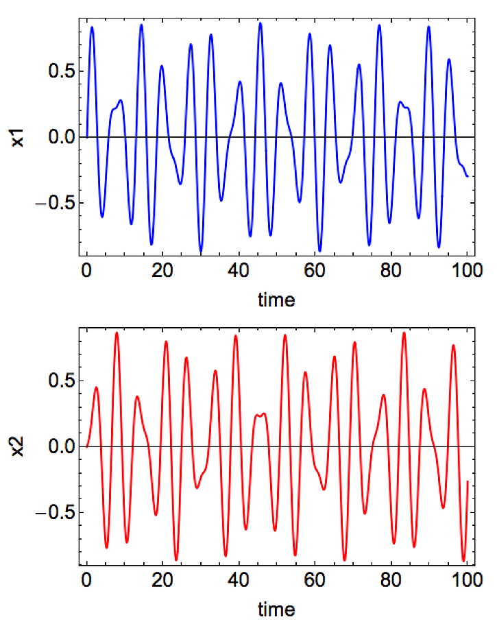
Neither \(x_1\) nor \(x_2\) looks anything like a regular sinusoidal function, as in the uncoupled case! Although if I squeeze my eyes, I can convince myself there are still some periodicities in those figures… It turns out that, instead of looking at \(x_1\) and \(x_2\) individually, we I should be looking at is \((x_1 + x_2)\) and \((x_1 - x_2)\):

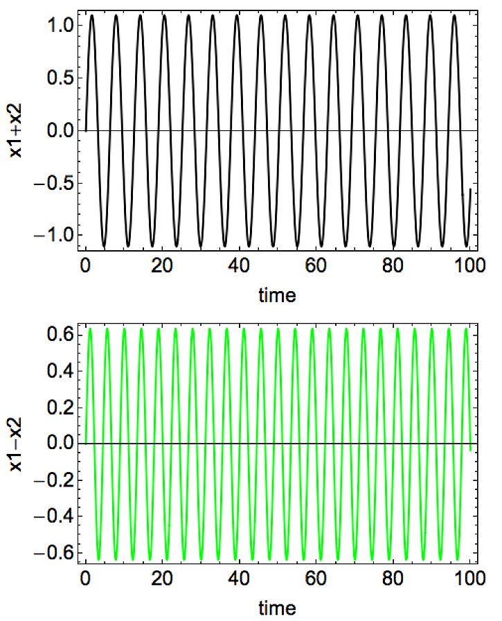
Voila! We now see the nice clean waves again, although with different frequencies.

The new quantities, \(y_1 = (x_1 + x_2)\) and \(y_2 = (x_1 - x_2)\), are called normal modes, and the corresponding frequencies are the eigen-frequencies of the system. Instead of looking at the seemingly arbitrary \(x\)s, one can get a much better grip of the system by looking at the \(y\)s. The wikipedia page actually do a pretty good job on describing what transformation should one do to go from \(x\)s to \(y\)s, but here I just want to have a visual confirmation, to reveal the value of the normal mode.

Update: found a terrific site with good lecture notes on this subject!