Comparing two ranked lists

There comes times when we want to compare two rankings, for example, between my top-5 list of all time best male distance runners, and that of my friend Robin. My top 1 through 5 are:

1. Kenenisa Bekele
2. Haile Gebrselassie
3. Paul Tergat
4. Emil Zátopek
5. Killiant Jornet

While Robin agrees mostly with me, but his top-5 list consists of:

1. Haile Gebrselassie
2. Kenenisa Bekele
3. Emil Zátopek
4. Killiant Jornet
5. Mo Farah

So the question is, how similar is my ranked list to Robin’s? As much fun as it is to rank distance runners, we encounter such problems in other cases, such as movie rankings, or product rankings. A similarity measure can be quite useful to help us to cluster customers, or to evaluate a ranked list generated by a new model to the old ones. But it is not quite straightforward to derive a numerical value, for example, between the two top-5 rankings shown above.

Before we dive in to find the proper protocols, it is best to enumerate some properties we like to have for the similarity measure.

First, we like it to be bounded, say, between [0, 1], with 0 meaning completely different and 1 meaning identical – we will further elaborate what does (in)different mean later.

Second, we like such protocol handle non-conjoint case, i.e., to allow items shown in only one of the two lists. In the example above, Paul Tergat is only in my list while Mo Farah is only in Robin’s list, but we should be able to handle such situations.

Third, we like to handle lists with different lengths, e.g., comparing a top-5 list and a top-10 list, or even more broadly, comparing results between two infinitely long lists (think search results of the same query returned by Google and Bing).

Now we have at least three desired properties in mind, we can seek for the appropriate measures. There are mostly two types of similarity measures between ranked lists: correlation based, and intersection based. One of the key difference between the two categories is that, the correlation based measures only works in the conjoint case, namely, item appears in one list must appear in the other list as well, but the intersection based method can handle the non-conjoint cases too.

An popular example for the first category is the Kendall’s tau, which has a nice probability interpretation. In short, if we randomly pick two items that are in both lists (say, Kenenisa Bekele and Haile Gebrselassie), Kendall’s tau is the probability that one (Kenenisa Bekele) ranks before (or after) another (Haile Gebrselassie) in both lists. This property nicely bounds Kendall’s tau between 0 and 1, however, the non-conjoint requirement (second desired property) would not be met, as in our example, due to (dis)appearance of Paul Tergat and Mo Farah. Of course, we can remove all those items that only appear in one list, re-rank the remaining ones, then calculate the Kendall’s tau, but it doesn’t sound like a satisfactory solution… In terms of running time: we are effectively counting the number of inversions, hence given two lists with the same length of \(N\), Kendall’s tau can be calculated in \(O(N \log N)\). Not surprisingly, scipy already has an implementation for Kendall’s tau.

Then comes the intersection based measure. The idea is very simple, we simply count what is the proportion of overlapped items, among all items, as we progress the ranking depth. Such proportion is also called Jaccard similarity. This will become clear in the figure shown below.

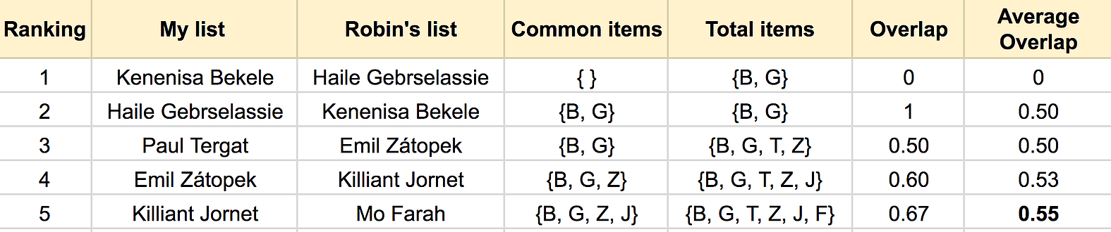
The figure above should be quite self-explanatory, in which I represent runners with the first letter in their last names. The overlap is the ratio between the length of common items set (intersection) and the total item set (union). The average overlap at each ranking depth \(k\), is the average of all the \(k\) overlaps. The last average overlap (0.55), will be our similarity measure. A similar metric based on this idea, called rank-biased overlap (RBO), is proposed in this paper.

Compared to the correlation based measures, the intersection based measures handily deal with the non-conjoint cases, hence satisfying our second requirement outline above. Furthermore the authors of RBO also made some modifications, to satisfy the other two requirements. RBO also comes with some other nice properties, such as the top-weightness: the (dis)agreement at the top of the two lists will weight more than the same (dis)agreement towards to the bottom of the lists, this is quite natural, isn’t it?

In terms of calculating the RBO, it could be done in \(O(N)\) time, where \(N\) being the length of the longer list. Here you can find my implementation of the RBO in python.