The fundamental problem of causal inference, part 1

What are we talking about?

Many companies spend large sums of money on marketing, including but not limited to, sending coupons, emails to some customers. It is almost true that one should not send the same message to all the customers. The reason is quite obvious: there is some unit cost associated each of the messages, either monetary or not (say, customer fatigue). For the sake of simplicity, let us assume the number of marketing messages is already determined (e.g., 5 million pieces), the central question then becomes: which 5 million from the total customer pool (say, 100 million)?

A very appealing method is to train certain propensity model, which takes in each customer’s attributes (age, gender, past shopping behaviors, etc.), and predict the probability that she will make a purchase (say, in next month). Once we have trained a reasonably good propensity model (evaluated with appropriate metrics), we then apply our marketing actions to those top prospects, to lock in their purchases.

However, such approach is fundamentally flawed, in that it completely disregards the effects of marketing actions. Even if we observe better performance from those customers who are treated with marketing actions, it will be mere correlation but not causation: how do we know whether they will behave the same if they are not treated?

In this post and next, I will try to illustrate how one can go about identifying the casuality, and build model to maximize the causal effects in, for instance, a marketing campaign.

Model to identify causal effects

The goal

The ultimate goal of any marketing action (campaign) is to change the recipient’s behavior. Furthermore, we like to quantify the word ‘behavior’: let us consider the simplest behavior – make a purchase. Then there are 4 possible outcomes after a customer has been treated with the marketing actions:

1. From not-shopping to shopping (persuadable);
2. From not-shopping to not-shopping still (lost cause);
3. From shopping to shopping still (sure thing);
4. From shopping to not shopping (do not disturb).

The above cases can be better understood with the figure shown below. Furthermore, we group the ‘lost cause’ and the ‘sure thing’ together as ‘in-different’, in the sense that our marketing action is indifferent to their behaviors.

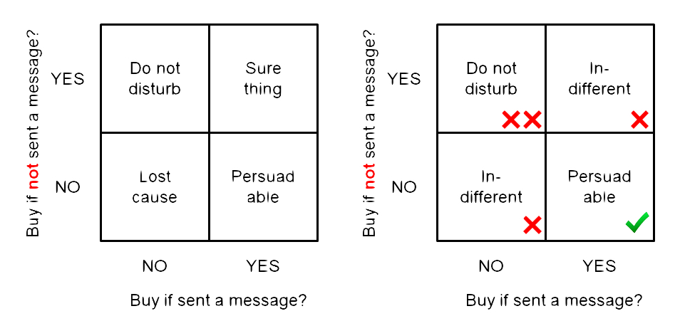
Clearly, the “persuadable”s are the subset of customers we want to identify and apply our marketing actions to. It is the job for us, to build models to identify them (and the “in-different”s and “do not disturb”s).

A black-box model

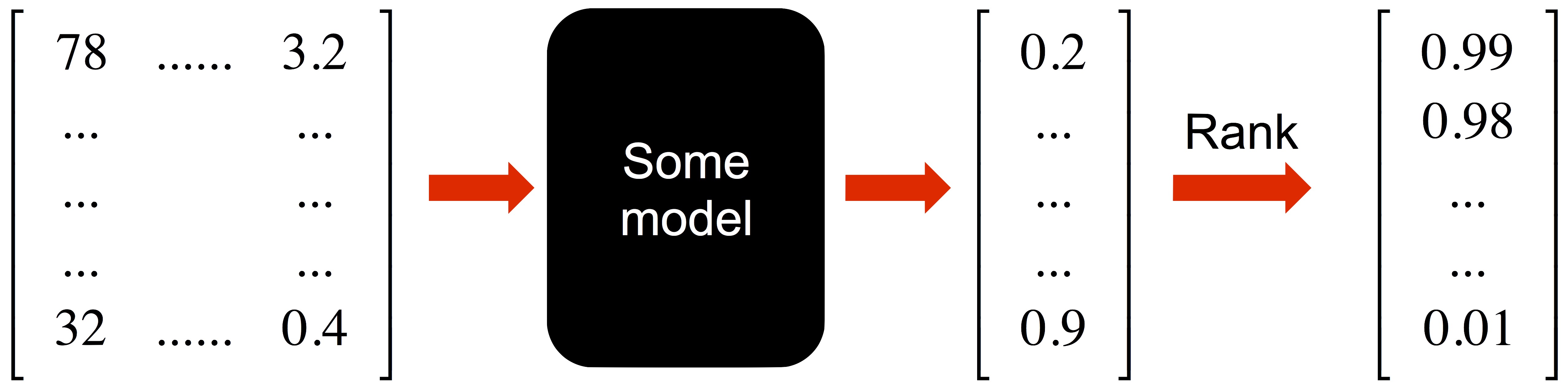
Let’s first imagine how such a model should work. The inputs to the model should be all our customers, expressed with certain features (e.g., total spend in previous 12 months, total number of store visits). If we have m customers, each expressed with n feature, then we can imagine the input to the model as a m x n matrix. After some number crunching, the model will assign a numerical score to each of the m customers (ideally a bounded score, say, between 0 and 1). A “persuadable” should have a higher score than an “in-different”, whose score is higher than a “do not disturb”. Then with the pre-determined budget constraint (e.g., 5 million coupons), we can just pick the top-k customers accordingly. Voila, we are done!

Then suddenly, you are handed two models, one of which just assign a random score to each customer, how can tell which one is better (hopefully not the random number generator)? Therefore, before we dive into model building, we first need to establish a meaningful evaluation metric. Unlike binary classification problem, such metric is not so obvious, due to the “fundamental problem of causal inference”.

The fundamental problem of causal inference (FPCI)

To make things simple, let’s think discretely for now: our goal is to categorize all our customers to one of the three categories (persuadable, in-different, and do-not-disturb). Imagine, for each customer, we first ask her: will you shop? Write down the answer (yes/no). Secondly, apply the marketing action to her (send her a coupon). Thirdly, we observe whether she comes to shop (yes/no). In this way, we are able to assign each of our customers to one of the three types. Of course, it is impossible for us to carry out such task, especially for the first step. There is just no way to learn a customer’s prior opinion / behavior explicitly. Without such knowledge, even we can observe her response (in the third step), there is no way for us to derive the causal relation.

Is there a fix for the above issue? How about in the second step, instead of applying the marketing action, we will do nothing, then in the third step, the observed response can be inferred as the customer’s prior behavior. This sounds very logical, however, the fallacy lies in that, one can not simultaneously apply and not apply the marketing action to the same person, unless someone invents a time machine. This is known as the “fundamental problem of causal inference, FPCI”. The time machine part is from me.

Per the same wikipedia article: “The FPCI makes observing causal effects impossible. However, this does not make causal inference impossible. Certain techniques and assumptions allow the FPCI to be overcome.” Here we will choose one of such techniques, and derive our evaluation metric from it.

Randomized treatment and control groups

The technique utilizes the randomization assignment of treatment (applying marketing action) and control (not applying marketing action) groups.

Recall that we can not treat / not-treat the same customer at the same time, since we don’t have a time machine, how about the next best thing, that we can clone the customer? Then we will treat the original, and not-treat the clone. However, it doesn’t seem we can do that either… Let’s take one more step back, how about find some other customer who is (almost) identical to the original? It should work, so long we can find such copies – one can imagine what a daunting task that would be!

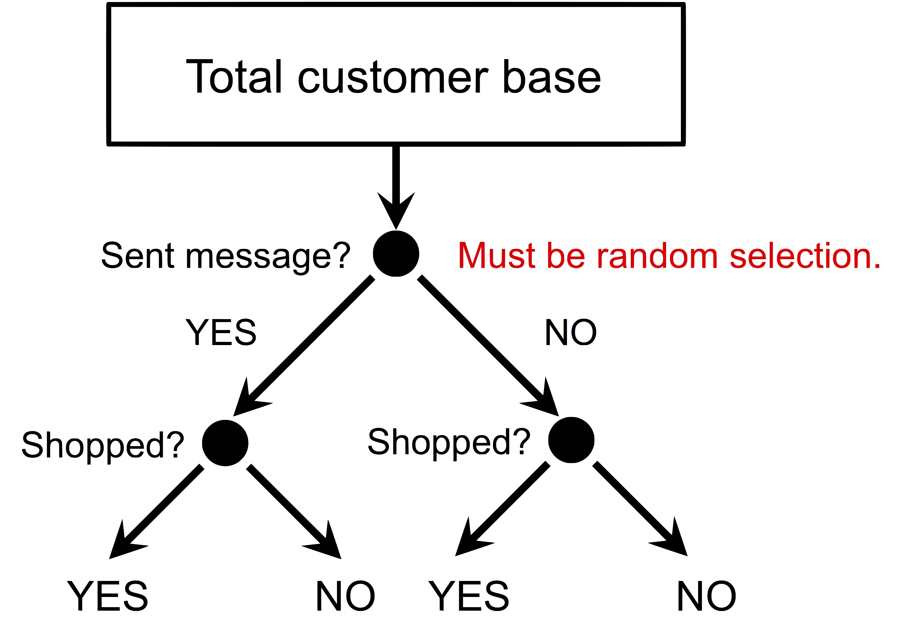
Let’s take yet one more step back: instead of studying each customer with her individual response, how about we study the averaged response from a group of customers. Doing so, we change the problem from finding two (almost) identical individuals, to finding two (almost) identical group of individuals. Here is where the randomization shines: given that our assignment is random (to either treatment or control group), if the size of each group is large enough, then we can safely say that these two groups are (almost) identical.

Then we apply our marketing actions to the treatment group, and do nothing to the control group, and observe their responses, as shown in the figure below.

We will have the results in, from both groups, how can we make sense of it? More importantly, can we use these results to evaluate a model? To illustrate this, let’s consider an extremely simple case as shown below.

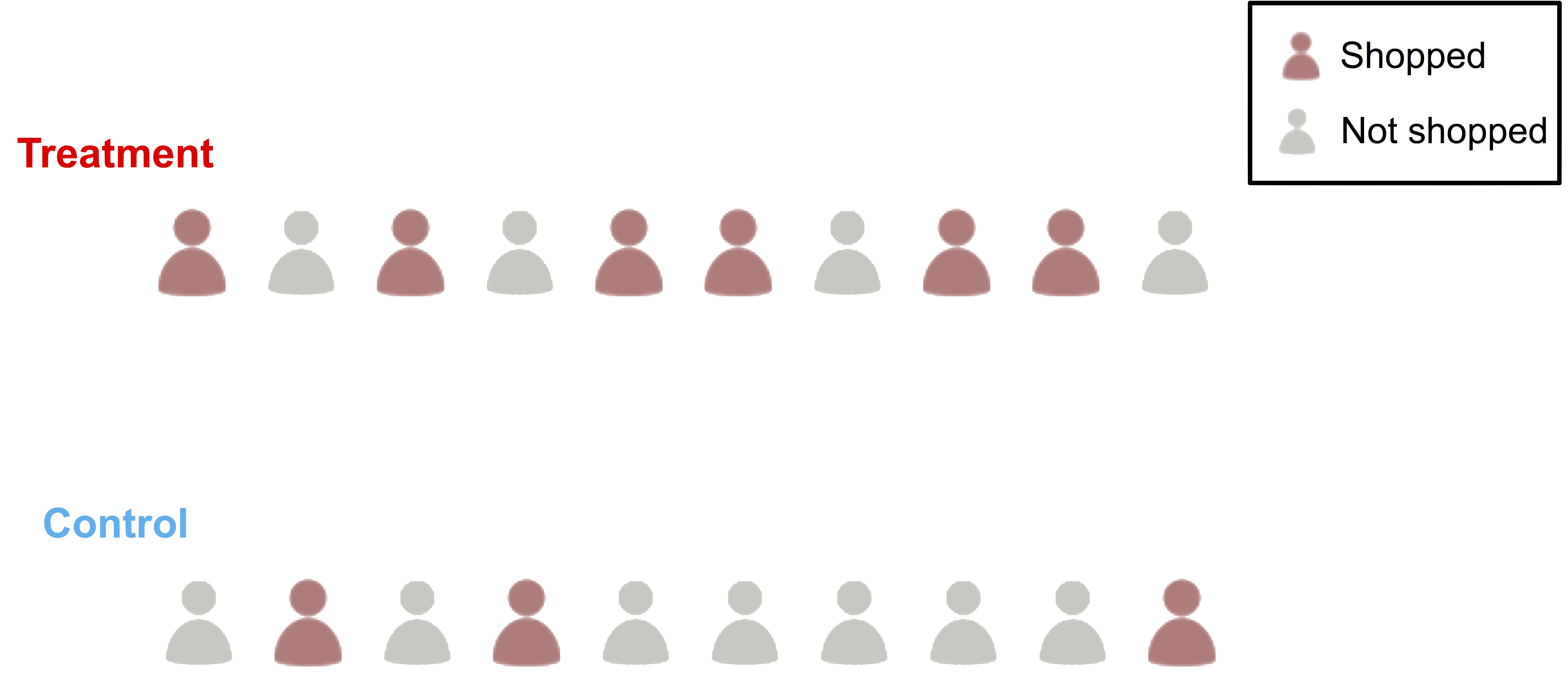
As we can see, both treatment and control groups consist of 10 people. Out of the 10 people in the treatment group, 6 come to shop; whereas only 3 people from the control group come to shop. Therefore, the response rate from the treatment group is 60%, higher than 30% from the control group. Recall that we consider the treatment group and control group are “identical”, except for the marketing action (the treatment). Hence we will attribute the observed difference to the marketing action, that is, the marketing action causes the difference of the response rate, and in this case, to our favor. We see an absolute lift (or uplift) of 30% in the response rate.

Evaluation metric

So far we don’t need any model, not even the black-box one. The random assignment gives us a 30% lift. However, can we do better than random? Imagine the company is going through some severe budget cut, and we can only apply marketing action to 5 customers. For the sake of simplicity, let us further assume that our total customer universe only contains the 10 people in the treatment group (what kind of company is that?!), then the question boils down to: which 5 to pick?

Now let’s consider how a model can help. First one up is the random number generator: it will just randomly pick 5 people, and since we are omniscient, we will know that the response rate will be 60% - it is still better than the baseline response rate of 30%!

Then another model can score the 10 customers (in the treatment group) in the fashion shown in the figure below. If we then pick the top-5 highest ranked customer to apply the marketing action, we will get a response rate of 100%! Talk about a smart algorithm!

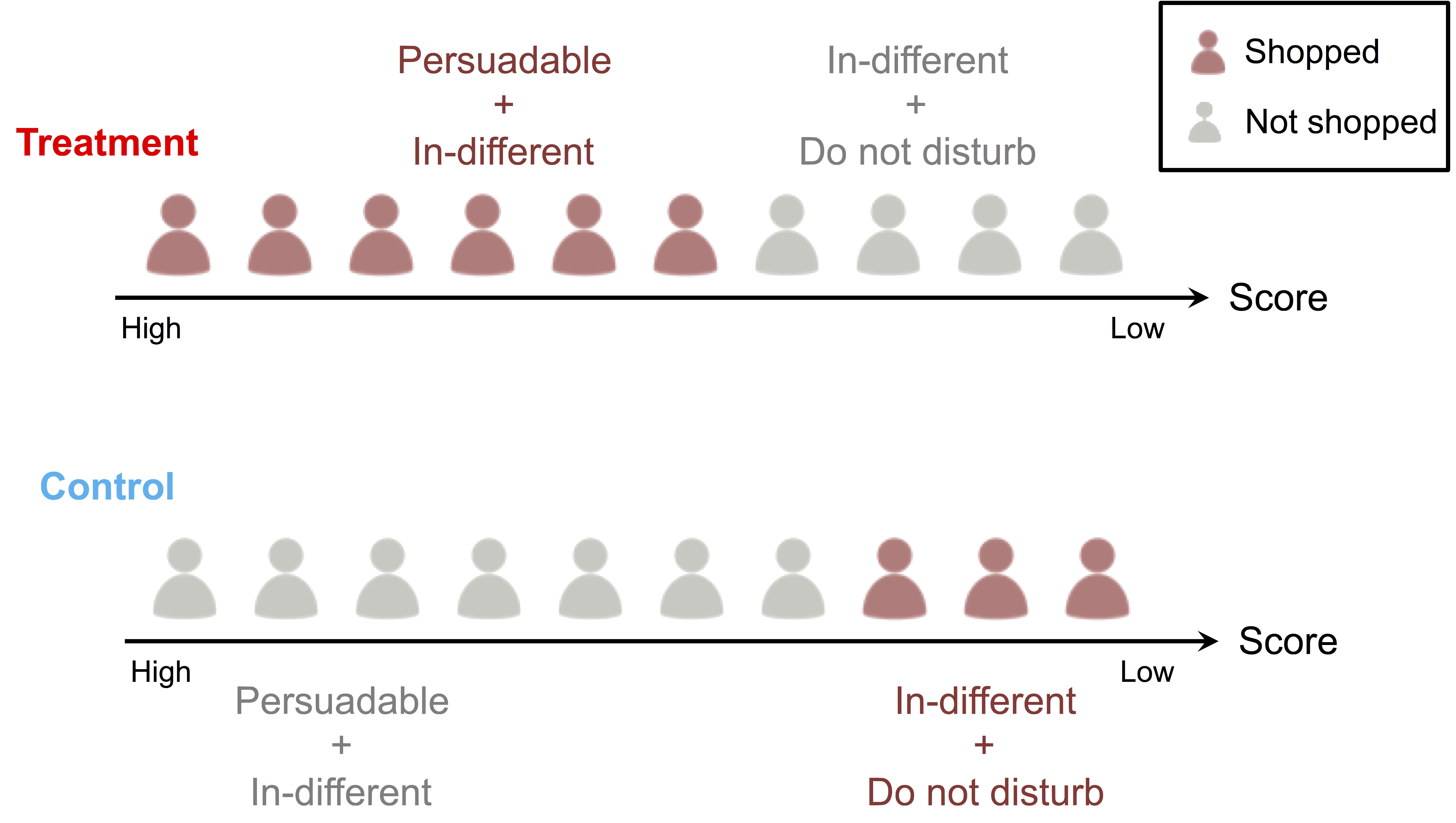
The same logic can be to applied to the control group: if a model can rank all the responded customers after those do not, that is the best we can ask for. Those responded customers do not need any marketing messages anyway.

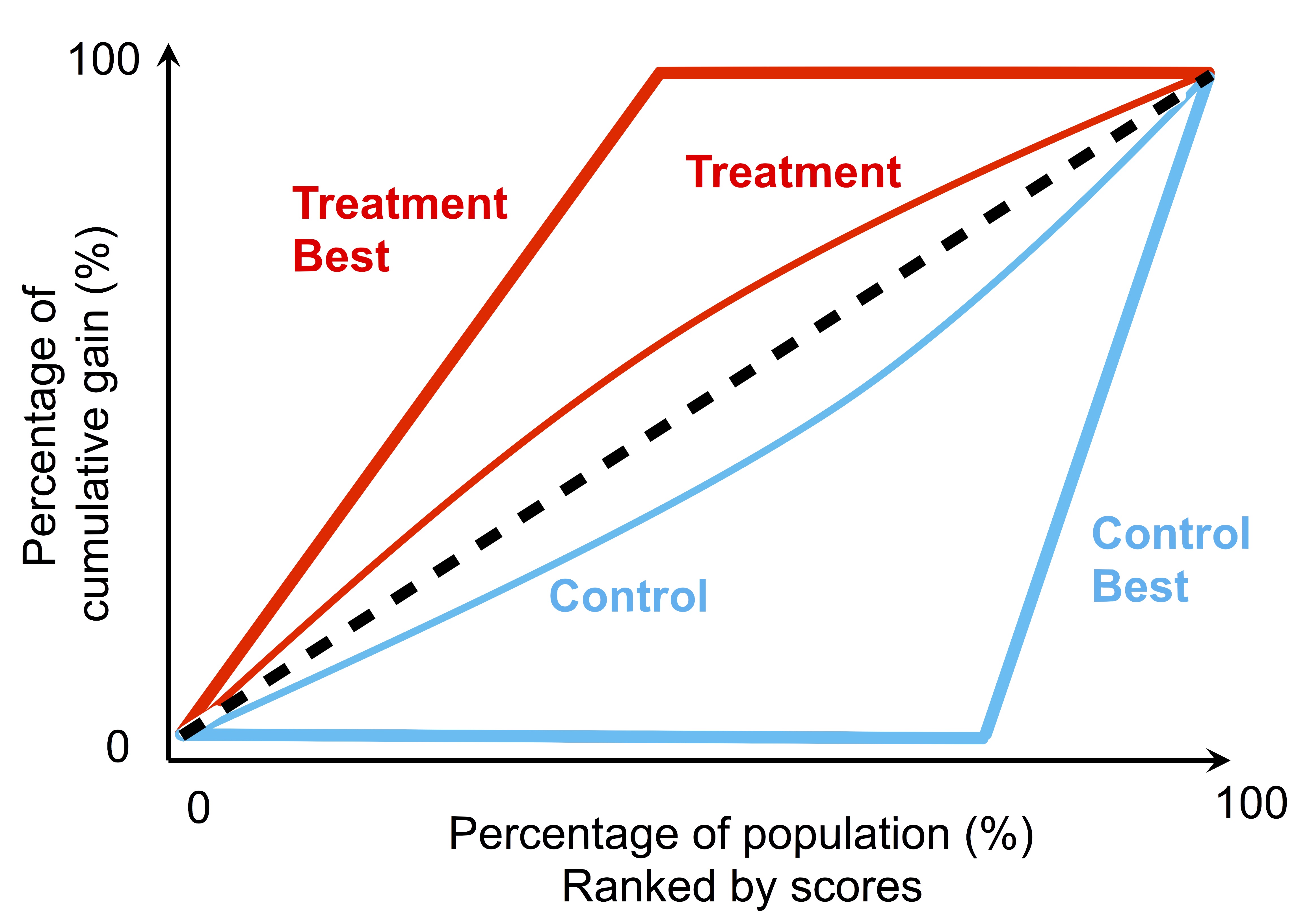
Once we understand the best-possible scenarios when applying a model to the treatment and control group, we can quantify such performance with a cumulative gain curve. A cumulative gain curve can be used to evaluate the performance of a binary classifier (similar to a receiver operating characteristic curve), and by plotting both the “best” treatment and control curves together with curves produced by real models, we can then evaluate how far off the model from the ideal case. For example, we can calculate the area between the treatment and control curve, and compare it to the ideal cases by taking ratios. This is similar to use normalized Gini coefficient to evaluate the performance of a binary classifier, therefore, let’s call this ratio as Q coefficient. The range of Q coefficient is bounded between -1 and 1, whereas larger value indicates better performance.

Finally, we arrive at a scheme (randomized treatment and control group), and the corresponding metric (Q coefficient) that we can use to evaluate any model that aims to answer FPCI. Now let’s build a model.

Conclusion

In this post, we first articulate the fundamental problem of causal inference (FPCI) with a simple marketing campaign example. We have arrived at one technique (randomized treatment and control groups) that can isolate the causal relation between actions and responses, as well as a convenient metric (Q coefficient) to evaluate a causal model. In next post, we will keep traveling along this line of thought, to explore how we can build model(s).