Fitting a Mixture of Gaussians

A little warm up

As a data scientist, we are dealing with various of distribution on an almost daily basis. The simplest (and the grandest) is undoubtedly the Gaussian (normal) distribution. Let’s assume that we draw 10,000 samples of adult American women’s weight (in the unit of lb.), shown in the figure below. By looking at it, we have every reason to believe it follows a Gaussian distribution, but we don’t know its mean nor its variance, how can we find out?

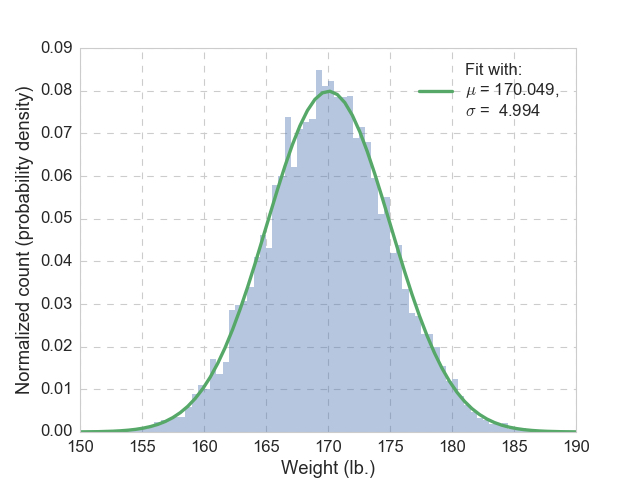
Well, that is easy, we will just use the mean of the 10,000 samples (sample mean) as the mean of the Gaussian distribution (population mean). Similarly, we will use the sample variance as the population variance. The resulting probability density function (pdf) is plotted in green, together with the histogram, and we see good agreement. The data are actually generated from a Gaussian distribution with mean of 170, and variance of 25, so our guesses are pretty close. But why this is the right way?

Maximum likelihood estimation

The reason is called the maximum likelihood estimation (MLE). As in most machine learning problems, we want to set up an objective function, and then tweak its parameters to maximize its value. In this case, we want to maximize the probability of observing all these (10,000) samples, by tweaking the assumed probability distribution’s (Gaussian) parameters (mean and variance). Here, we define the likelihood function (with the Gaussian distribution) as:

\[\begin{eqnarray} \mathcal{L}_i(x_i; \theta) &=& P(x_i | \theta) \\ &=& \frac{1}{\sqrt{2\pi\sigma^2}} e^{-\frac{(x_i - \mu)^2}{2\sigma^2}}, \end{eqnarray}\]

where \(x_i\) is the sample under consideration, and \(\theta\) represents the parameters of the assumed distribution. In our case of Gaussian distribution, we have \(\theta = (\mu, \sigma^2)\). If there are \(N\) independent samples, then the objective function, namely, the probability of observing the \(N\) samples, \(\mathcal{L}(X; \theta)\) is simply the product of all the individual likelihoods:

\[\begin{eqnarray} \mathcal{L}(X; \theta) &=& \prod_{i=1}^{N}\mathcal{L}_i(x_i; \theta) = \prod_{i=1}^{N} P(x_i | \theta) \\ &=& {\Big(\frac{1}{\sqrt{2\pi\sigma^2}}\Big)}^N \prod_{i=1}^{N} e^{-\frac{(x_i - \mu)^2}{2\sigma^2}}. \end{eqnarray}\]

In practice, one usually considers the logarithm of the objective function, as \(\ell(X; \theta) = \ln{\mathcal{L}}(X; \theta)\), since \(\ln{()}\) is a monotonically increasing function, we do not lose any generality. Then we transform the objective function from likelihood to log-likelihood as:

\[\begin{eqnarray} \ell(X; \mu, \sigma^2) &=& \sum_{i=1}^N \ln{P(x_i | \mu, \sigma)} \\ &=& -\frac{N}{2}\ln{(2\pi\sigma^2)} - \frac{1}{2\sigma^2}\sum_{i=1}^N(x_i - \mu)^2. \end{eqnarray}\]

Again, here \(\theta = (\mu, \sigma^2)\). To find the maximum of \(\ell\), we bring out our favorite method to find an extremum, namely, solving \(\mu, \sigma^2\) for \(\partial \ell / \partial \mu = 0\), and \(\partial \ell / \partial \sigma^2 = 0\). This is high-school level calculus, hence we have:

\[\begin{eqnarray} \mu &=& \frac{1}{N}\sum_{i=1}^N x_i,\\ \sigma^2 &=& \frac{1}{N} \sum_{i=1}^N (x_i - \mu)^2. \end{eqnarray}\]

We can further prove that with this values of \(\mu\) and \(\sigma^2\), we actually have the maximum of \(\ell(X; \mu, \sigma^2)\). Therefore, MLE justifies our “fitting” procedure.

How about gradient descent

Before we move on, how about that gradient descent method to calculate the maximum value? Sure, we can randomly pick a set of initial values for \(\mu\) and \(\sigma^2\), and then follow the standard recipe of gradient descent to find the maximal \(\ell\) and the corresponding \(\mu\) and \(\sigma^2\), but then we have to deal with the proper choices of initial values, learning rates (and its decay), etc. I actually implemented a vanilla version of gradient descent on this problem, only to tune the learning rate carefully to make it coverage, yikes! Since we already have such an easy way, why bother?

So what have we learned? Here we are given a set of data (10,000 weights for adult women), and an assumed type of distribution (Gaussian), we are able to “learn” the parameters of the distribution (mean and variance) from the data using MLE. Therefore, if we are presented with a new sample from the same population, we are able to make statistical inference. Really nothing fancy.

Mixture of two Gaussians

Let’s make things a bit more interesting: instead of \(N\) = 10,000 weights of adult women, we are given \(N\) = 30,000 weights of adult women and men, and the histogram of these 30,000 samples looks like the figure below.

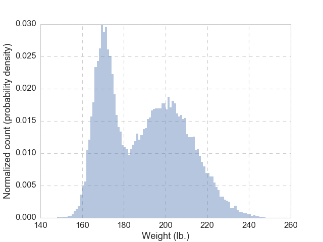
Clearly, there are two humps, and very likely, one is made up of women and the other one of men. Now let’s ask this question: given someone with a weight of 180 lb., how likely this is a male, \(M\) (or a female, \(W\))?

What do we need to learn

The question can be rephrased as, given a data point (\(x_i\)), what is the probability that it is drawn from one class (e.g., \(M\)). Written in equation, we are asking for \(P(M|x_i)\). Naturally, we like to apply Bayes’ rule here:

\[\begin{eqnarray} P(M|x_i) &=& \frac{P(x_i|M)P(M)}{P(x_i)} \\ &=& \frac{P(x_i|M)P(M)}{P(x_i|M)P(M) + P(x_i|W)P(W)}. \end{eqnarray}\]

In order to answer this question, we need to know all the elements in the above equation. Like in the previous case, we assume that both the men’s weight and women’s weight follow their respective Gaussian distributions, parameterized by \(\mu_M, \sigma^2_M\) and \(\mu_W, \sigma^2_W\). Once we know that, the likelihood calculation would be straightforward. Furthermore, we need to know the priors, namely, the proportional of each gender (\(\pi_M = P(M)\), and \(\pi_W = P(W)\)). With these 6 parameters (or 5, since \(P(M) + P(W) = 1\)), we can fully describe this mixture of Gaussians, and answer the question. We need to learn all of that from the data.

The objective function

The game plan is still the same: construct a proper objective function that is parameterized by \(\theta = (\mu_M, \sigma^2_M, \mu_W, \sigma^2_W, \pi_M, \pi_W)\), and then tweak \(\theta\) to maximize the objective function’s value.

Naturally, the objective function is again the log-likelihood function, \(\ell\), as:

\[\begin{eqnarray} \ell(X; \theta) &=& \sum_{i=1}^N \ln{P(x_i|\theta)} = \sum_{i=1}^N \ln{P(x_i|\mu_M, \sigma^2_M, \mu_W, \sigma^2_W, \pi_M, \pi_W)} \\ &=& \sum_{i=1}^N \ln{\big[\pi_M P(x_i|\mu_M, \sigma^2_M) + \pi_W P(x_i|\mu_W, \sigma^2_W)\big]}. \end{eqnarray}\]

Well, this is similar to the single Gaussian case, can we apply the same calculus trick? Not quite… the addition inside the \(\ln{()}\) makes things difficult if not impossible. So, we need a plan B (and hold off the urge of using the vanilla version of the gradient descent just for a bit).

The hidden (latent) variable

So the addition is the killer, can we get rid of it? What if for each \(x_i\), we know its gender (i.e., class), call it \(z_i\), to be \(W\) or \(M\)? If we are geared with such information, then for each \(x_i\), all terms inside the \(\ln{()}\) but one will vanish, then we are back into our comfort zone! Accordingly, the objective function (log-likelihood) becomes:

\[\begin{eqnarray} \ell(X; \theta, Z) &=& \sum_{\substack{i=1 \\ z_i=M}}^N \ln{\big[\pi_M P(x_i|\mu_M, \sigma^2_M)\big]} + \sum_{\substack{i=1 \\ z_i=W}}^N \ln{\big[\pi_W P(x_i|\mu_W, \sigma^2_W)\big]}\\ &=& \Big( \sum_{\substack{i=1 \\ z_i=M}}^N \ln{\big[P(x_i|\mu_M, \sigma^2_M)\big]} + \sum_{\substack{i=1 \\ z_i=W}}^N \ln{\big[P(x_i|\mu_W, \sigma^2_W)\big]} \Big) \\ &~& + \Big( \sum_{\substack{i=1 \\ z_i=M}}^N \ln{\pi_M} + \sum_{\substack{i=1 \\ z_i=W}}^N \ln{\pi_W} \Big). \end{eqnarray}\]

Hooray! No additions inside \(\ln()\)! Now we get all the ducks lined up in a row, ready for us to take derivatives, assuming that we know the value of \(Z\) (the vectorized version of all \(z_i\)’s). But \(Z\) is hidden from us (not observed), thus it bears the name of latent variable. To deal with that, we need the EM algorithm, not Maxwell’s EM, but the Expectation-Maximization.

Before we move on, let me do some re-organization of the symbols, to prevent the equations from getting even longer. First, let’s abstract the gender as class. Clearly, we are dealing with 2 classes here, and I will map the subscript \(M\) to 1, and \(W\) to 2. Next, I will introduce the indicator function \(\textbf{1}()\) to make things concise. With these modifications, the log-likelihood for our mixture of two Gaussians becomes:

\[\begin{eqnarray} \ell(X; \theta, Z) &=& \sum_{i=1}^N \sum_{j=1}^2 \textbf{1}(z_i=j) \big(\ln{P(x_i|\mu_j, \sigma^2_j)} + \ln{\pi_j} \big) \end{eqnarray}\]

Remember that we are interested in values of \((\mu_j, \sigma^2_j, \pi_j)\) that maximizes \(\ell\), so let’s expand \(P(x_i | \mu_j, \sigma^2_j)\) and take derivatives to get:

\[\begin{eqnarray} \mu_j &=& \frac{\sum_{i=1}^N\textbf{1}(z_i=j) x_i} {\sum_{i=1}^N\textbf{1}(z_i=j)},\\ \sigma^2_j &=& \frac{\sum_{i=1}^N \textbf{1}(z_i=j) (x_i - \mu_j)^2} {\sum_{i=1}^N \textbf{1}(z_i=j)},\\ \pi_j &=& \frac{1}{N} \sum_{i=1}^N \textbf{1}(z_i=j). \end{eqnarray}\]

Few things to notice here. First, the solution for \(\pi_j\) is subjected to the constraint that \(\Sigma_{j=1}^2 \pi_j = 1\), hence, it is obtained by using Lagrange multiplier. Second, this framework can be extended to \(k\) > 2 classes, as well \(d\) > 1 dimensions. In the latter case, we need to switch to matrix representations.

Expectation-Maximization

We see that, we can maximize the log-likelihood function rather easily, if we know the values of all \(z_i\)’s. Sadly, we only observe \(x_i\)’s, but not \(z_i\)’s. What can we do? Hummm…. how about just guessing?

Why not? In our running example, for each weight we observe, let’s also flip a coin, to assign a randomly guessed gender to that person. Then we proceed to calculate the maximal \(\ell(X; \theta, Z)\) as outlined above. Problem solved. But the guessing part is still lingering: what if we start out guessing differently? Or alternatively, we if we can guess better?

Expectation: improving guesses

Indeed we can improve our guess. The critical piece is that: instead of assigning “hard” values to \(z_i\) (0 or 1), we will do a “soft” assignment to \(z_i\), let it represents the probability of sample \(x_i\) is drawn from class \(j\). Given this paradigm change, we change the latent variable from \(z_i\) to \((w_{i1}, w_{i2})\), with the constraint that \( \Sigma_{j=1}^2 w_{ij} = 1 \). Effectively, \( w_{ij} = P(z_i = j) \). The hard assignment corresponds to the special case that \(w_{ij} \in (0, 1)\).

Once again, we will invoke Bayes’ rule, since we need to update our belief from the prior (i.e., previous guesses of \(w_{ij}\)), with the likelihood under this prior belief. Put that into equations, the improved guess are:

\[\begin{eqnarray} w_{ij} = P(z_i = j | X; \theta) &=& \frac{P(x_i | z_i=j; \theta) P(z_i = j)} {P(x_i; \theta)} \\ &=& \frac{P(x_i | z_i=j; \theta) P(z_i = j)} {\sum_{j=1}^k P(x_i|z_i=j; \theta) P(z_i=j)}. \end{eqnarray}\]

Here, \(P(z_i = j)\) is the prior belief, namely, the previous guess.

Maximization: the old MLE

Let’s not lose sight of our goal: to find \(\theta\) that maximize the log-likelihood \(\ell\). Previously we have found the recipe to calculate \(\theta\) based on known, albeit guessed, hard assignment of \(w_{ij}\)’s. Now we have a better guess of, soft assignment, \(w_{ij}\)’s, let’s re-calculate \(\theta\) in a similar fashion, hoping that it will give larger \(\ell\). The only change is to replace the discrete weights (by indicator function), with \(w_{ij}\)’s, as:

\[\begin{eqnarray} \mu_j &=& \frac{\sum_{i=1}^N w_{ij} x_i} {\sum_{i=1}^N w_{ij}},\\ \sigma^2_j &=& \frac{\sum_{i=1}^N w_{ij} (x_i - \mu_j)^2} {\sum_{i=1}^N w_{ij}},\\ \pi_j &=& \frac{1}{N} \sum_{i=1}^N w_{ij}. \end{eqnarray}\]

Notice that, here we use results from the Expectation step, namely, values of \( w_{ij} \)’s. In the meantime, the results obtained from here (Maximization step), namely, (\( \mu_{j}, \sigma_{j}^2, \pi_{j} \))’s can be used to update \( w_{ij} \)’s. This naturally imply an iterative algorithm, aiming to maximize \(\ell\), which is our ultimate goal.

Correctness and convergence

The EM algorithm seems intuitive, with the help of the latent variable. But is it correct? If it is correct, will it converge? The answers to both questions are yes. The proof can be found from this nice note by Andrew Ng. At the heart of it is to apply Jensen’s inequality on the \(\ln()\) function, which makes our objective function (log-likelihood).

As an iterative algorithm, EM suffers from the pitfall that it is not guaranteed to find the global maxima. But often time we would be happy with a good enough local maxima. From a more general viewpoint, we can treat the Lloyd’s algorithm for k-means clustering as a special case of EM algorithm, with hard assignments and zero variance.

Finally, how about finding maximum log-likelihood with gradient descent? One surely can, and maybe with faster speed. However, as there are many knobs to turn in the gradient descent process, EM algorithm can be implemented more easily, with clear narratives.

He or she?

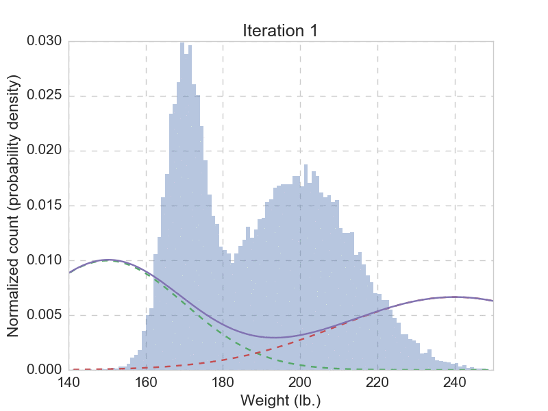
Talk is cheap, we need to see that EM algorithm actually works. Of course we do. Remember the question that got us started? We need to fit the 30,000 weights with a mixture with two Gaussian distributions, using the EM-algorithm outlined above. Here you can find a quick implementation of this use case, and the animation below shows the fitting result from the first 20 iterations.

After we have let the EM algorithm converge, we get the final parameters as: \(\mu_1 = 170.032\), \(\sigma_1 = 4.957\), \(\pi_1 = 0.331\), and \(\mu_2 = 199.862\), \(\sigma_2 = 15.052\), \(\pi_2 = 0.669\). Now we can comfortably answer the question: if someone is drawn from the same population, with a weight of 180 lb., then there is 0.322 probability being a he, and a 0.678 probability being a she. This seems reasonable, given that there are more women than men in the given population. Unlike hard assignment methods such as k means, here we give a probabilistic answer, which is more natural.