k nearest neighbor search, without brute force

This is an easy task

I was inspired by a co-worker’s project to look into this problem. In her particular case, she has two sets of data, let’s call them the query set \(Q\), and the target set \(T\). Both sets contain data of same dimension \(d\), and there are \(M\) and \(N\) samples in \(Q\) and \(T\), respectively. In essence, we can treat the set \(Q\) as a \(M \times d\) matrix, and similarly, the set \(T\) as a \(N \times d\) matrix.

Then here is the task: for each sample \(q \in Q\), we want to find out the 5 samples from \(T\), such that, no other sample from \(T\) has distance between itself and the query point is closer than those 5 samples. In another word, we want to find the 5 nearest neighbors (5-NN) of \(q\) in \(T\). The value of 5 here is rather arbitrary, and it can be generalized to k-NNs. More generally, we want to do the nearest neighbor search.

Let’s consider a very simple case to visualize the essence of this problem, that is, take the dimension \(d\) as 2. Let’s also define the distance between any two samples as the simple Euclidean distance. By doing so, we can draw those samples as points in the 2-D plane, and the distance between two samples is just, well, distance. Furthermore, let’s assume \(M\) = 1 and \(N\) = 100. Then this problem is reduced to: given 100 points on a 2-D plane, and a query point \(q\), what are 5 nearest neighbors of \(q\)?

One can probably solve this problem in less than 5 minutes, with few lines of python codes. Well, this is an easy task. Will the code run fast? Let’s see… Calculating the Euclidean distance takes \(O(d)\) time. For one query point, we will have to calculate the distance between itself and all points in \(T\), in which there are \(N\). So the total time budget for one query point is \(O(dN)\). If there are \(M\) query points, we will repeat above step \(M\) times, then the total time complexity will be \(O(dMN)\). In the end, we are doing a double for-loop. What’s more, this is just to find the nearest neighbor (1-NN): what if we want to find the k nearest neighbors (k-NN)? One can simply do the 1-NN search k times, then the total time budget is \(O(dMNk)\).

Is this time budget bad? If we are not dealing with high-dimension data, such as natural language problems, then we can consider \(d\) on the order of hundreds. But we might, and most likely will, have a lot of data: both \(M\) and \(N\) can be run into the order of millions. For my colleague’s problem, both \(M\) and \(N\) are about 100,000. We implemented the naive double for-loop algorithm, and the estimate run time is about 20 days!

A small boost

We came back to the drawing board… We also should probably use numpy more, and vectorize the data better, but still, there must be a better way, algorithmically.

Notice that, for k-NN, we want to maintain a list of k smallest values, as we are searching through all \(N\) samples in the set \(T\). So we could probably get a balanced binary search tree to store the k nearest neighbors seen so far, using their distance to the query sample as the key. In this way, we could cut the 1-NN search time from \(O(dNk)\) to \(O(dN\log{k})\). This is good, but given that \(k\) is usually not that big (as to \(M\) or \(N\)), we are only getting a small boost.

Can’t we learn a thing or two?

The brute force double for loop seems to be the deal-breaker. Let me mentally walk through the process again. First, we pick a query point from \(Q\), compare it against all the \(N\) points in \(T\), finding the 1-NN (or k-NN) for this query point. Next, we pick the next query point, and dive back to \(T\) again, until we exhaust all the points in \(Q\). But can we learn anything from the previous run in \(T\), such as, how the points in \(T\) are distributed? So when we are presented with a new query point, we can find our way in \(T\) more smartly, namely, bypass some points in \(T\) altogether?

Let’s make a map (or plant a tree)

It seems what we need is a map of \(T\), or algorithmically speaking, a data structure to describe \(T\). Of course, someone has solved this problem, and a typical data structure for this instance is called k-d tree. Here “k-d” stands for k-dimensional. Don’t confuse this k with the k in our k-NN notation. In this post, we use d to denote the sample dimension, we will stick to this d notation, and use k as in k-NN.

How to make a map? Let’s go back to our simple 2-D example: with all the 100 points form \(T\) shown on the xy-plane, we can draw a vertical line that separates them to two partitions, with some points on each side. Let’s assume this line bisects the xy-plane at about x = 0. Then if the query point lies at the far right side, then we probably don’t have to visit the points on the left-half of the xy-plane.

But probably is not good enough, how can we be sure? The key step is to draw a “bounding box” that contains all the points in each space partition. By making such a box, we can also measure the distance between the query point to the bounding box of the left partition. We can keep dividing each partition, until reaching some stopping criterion. For each partition, we will also make the corresponding bounding boxes. In this way, we make a map of \(T\), by making a binary tree out of it.

With this piece of information, the 1-NN query step becomes:

1. Make the “map” (make the k-d tree).
2. Given the query point, find out which partition is it in (traverse the k-d tree to the leaf that contains the query point).
3. Calculate the distance between the query point and all ohter points in the same partition (leaf). Remember the nearest neighbor, and the minimum distance.
4. Calculate the distance between the query point and the bounding box of the “sibling” partition (the other leaf under the same parent node). If this distance is larger than the minimum distance, then we can skip this “sibling” partition altogether. Otherwise, we will have to visit all the points in this sibling partition, and update the 1-NN if needed.
5. Once we have done with this sibling partition, we will traverse up along the tree, and then check the “uncle” partition (and possibly its children). We will keep traversing the k-d tree in the same fashion, until all the points in \(T\) are covered.

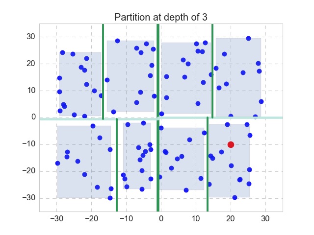
Nothing works better than a simple example. Let’s recall the 2-D case, as shown in the figure above. Here the k-d tree (or 2-d tree) has a depth of 3, as the space is partitioned by the mean value of alternating dimensions. In this case, the first partition is split with respect to the x-dimension, and separates the xy-plane to left and right, with the dark green line. We will make the bounding box for both of the partitions (not shown here). Then for each partition, the next partitions is split with respect to the y-dimension, with the split lines shown in light green. Again, we will make 4 bounding boxes (not shown). The next split will be taken with respect to the x-dimension again, on the 4 partitions, with thinner split lines shown in dark green again. Make bounding boxes, 8 of them this time. Now we have reached our pre-specified stopping criterion (depth equals to 3), so we stop, and the last 8 bounding boxes are also shown. We have finished the step 1.

Now we are handed the query point, which is shown in red. We will follow step 2 to 5 as described above, to get its exact 1-NN. In this particular case, it is apparent that we only have to visit the 11 points in the same depth-3 partition as the query point, as opposed to all the 100 points, and the nearest neighbor is the point at the lower left to the query point.

How fast is it

Yes! We see that by learning something about \(T\) through building a k-d tree, we can in practice greatly speed up the query. Actually, on average, the time complexity for 1-NN search is \(O(d\log{N})\) (hopefully with the example, this makes intuitive sense). So for the total \(M\) query points, the total search time complexity for 1-NN search will be \(O(dM\log{N})\). This is a huge boost!

How does it work in our case? Of course, the mighty scikit-learn has already taken care of the API, so we just need to be happy clients. It took only about 10 seconds to get the all the 5 NN for the \(M\) samples. WOW!

There is no free lunch

This is almost too good to be true, and of course it is. Although we achieved a huge gain in querying time, it takes time (and space) to build the k-d tree. Roughly speaking, it will take \(O(N\log{N})\) time and \(O(N)\) space to build the k-d tree. This doesn’t sound too bad… However, things can get quite ugly in high dimension case (\(d \sim N\)). As a rule of thumb, k-d tree works well if \(N \gg 2^{d}\). In high dimension case, one might want to consider inexact methods such as locality-sensitive hashing.

While making this post, I got interested in coding up the recursive partition of k-d tree, which leads to the figure shown in the post. You can find the full script here. In this case, the k-d tree is partitioned by the mean value of alternating dimensions. One can partition the sample space in any other manner, whereas the optimal partition protocol will depend on the distribution of the samples.