Machine Learning Design Patterns: Model Training

As I continue reading the Machine Learning Design Patterns book, in this post, I would like to summarize the takeaways from the Model Training section (Chapter 4). Most of the discussions are based under the neural network (NN) setting.

Useful Overfitting

In almost all cases, overfitting is a bad thing, since we usually build models with the presence of noise. Overfitting means we are learning the noise which is inherently random. However, there are noise-free situations, such as using an ML model to solve non-tractable deterministic problems (e.g., partial differential equations, chaotic systems), in such cases, overfitting is actually the desired behavior.

Aside from the above, less common, tasks, (intentional) overfitting can useful in general-purpose ML problems as well. When working on a new problem, one can (and should) intentionally overfit the model on a small subset of the data (e.g., one batch), to ensure the model is sophisticated enough to handle the full data volume. This seems to be a good practice that comes with no cost.

Checkpoints

This design pattern suggests saving the full model states periodically during the model training process. Here we have two questions need to be answered: what do we mean by full model states, and how often is considered appropriate for periodically.

Full model state v.s. model artifact

When we say model artifact, it is referred to the information needed to make inference, such as the NN architecture and weights. On the other hand, the full model state, will not only include the model artifact, but also information needed to perform the next iteration of the model training. The difference becomes crystal clear if one encounters hardware failure during training, which is not uncommon for NN models taking hours or days to train. Having merely the model artifact will not allow one to resume training, since we also need to know what is the current batch/epoch, learning rate (if we are following a schedule). For recurrent NN, we might also need to know the history of previous input values.

Batch, virtual epoch, epoch

Then let’s save the full model states (checkpoints) as often as possible! The atomic unit in NN model training is a batch, so why not export the model state after each batch? The problem is that such frequent snapshot will bring heavy disk I/O overhead, and increase the total training time. For example, if we have 16 million samples, and with a batch size of 32, there will be half million checkpoints to save for just one epoch!

The next natural choice is to save the checkpoints after each epoch. Although logically sound, it might not be optimal when dealing with large dataset. For such cases, one could probably only go through the full dataset a few iterations (epochs), and the resulting sparse checkpoints would not serve its purpose well.

The trade-off is what is called virtual epoch. To do so, one specifies: 1) the total number of iterations over a single sample (can be non-integer), 2) the total number of checkpoints, 3) batch size. With that, we can calculate the total number of steps (virtual epochs) for the full training, and each virtual epoch will contain multiple batches. We will then save checkpoints after each virtual epoch.

NUM_TRAINING_EXAMPLES = 1000 * 1000
STOP_POINT = 14.3
TOTAL_TRAINING_EXAMPLES = int(STOP_POINT * NUM_TRAINING_EXAMPLES)
BATCH_SIZE = 128
NUM_CHECKPOINTS = 32
steps_per_epoch = (
  TOTAL_TRAINING_EXAMPLES // (BATCH_SIZE * NUM_CHECKPOINTS)
)

How checkpoints can help

Aside from the benefit described above, checkpoints saved after each virtual epoch can speed up the retraining with newer data, effectively providing a warm start state as more recent data are added, as illustrated in the figure below.

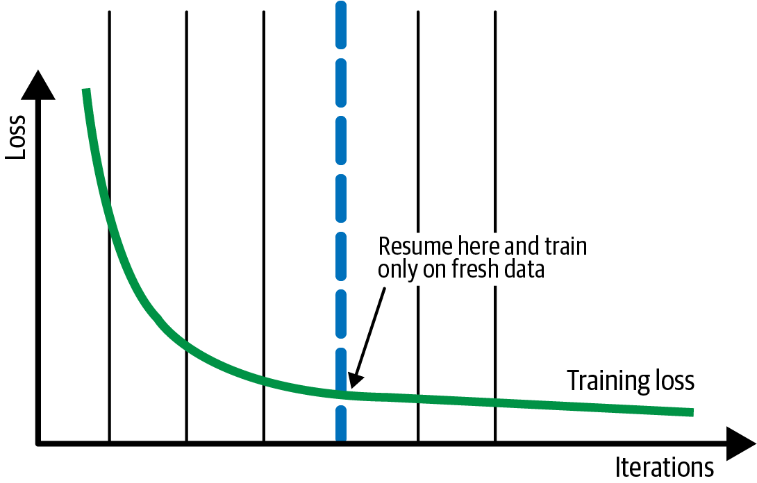
Another benefit of a more granular look of the training progression (with properly chosen virtual epoch size) is, we can examine the evolution of the loss to better locate the minimal, in the face of noise, and to apply regularization.

Transfer Learning

This design pattern is mostly used in the context of image of text models, where you can apply a similar task to the same data domain, but not so much for tabular data, as there are potentially infinite number of possible prediction tasks and data types. Since my works have mostly in the latter camp, I skim through this part rather quickly.

Distribution Strategy

Nowadays, it is common for a large NN model to have millions of parameters and massive amount of data to train on, for good reasons (better model performance). However, this inevitably increases the computation resources required, and time needed to train such models. Distribution Strategy aims to parallelize model training by utilizing multiple workers, to reduce the total training time.

Data parallelism versus model parallelism

Since stochastic gradient descent (SGD) only process one batch at a time to update the gradients, one can distribute data across different workers, and this is the essence of data parallelism. In model parallelism, the model is split and different workers carry out the computation for different parts of the model. The former is more intuitive and generally easier to implement.

Synchronous versus asynchronous

For data parallelism, a key question is how to coordinate the updates from different workers. There are two strategies: synchronous and asynchronous updates.

In synchronous training, the workers train on different slices of data in parallel, and the gradient values are aggregated at the end of each training step. This is performed via an all-reduce algorithm: each worker (CPU or GPU) has the same copy of the model, and SGD is performed on each worker with their share of the data. Once the locally updated gradients are computed, they are sent back to a central server to be aggregated (for example, averaged), so to produce a single gradient update for each parameter (hence an updated model). This updated model is then broadcasted to all workers for the next iteration.

In asynchronous training, the workers train on different slices of the data independently, but the model parameters are updated asynchronously, typically through a parameter server architecture. This means that no one worker waits for updates to the model from any of the other workers.

The trade-off between synchronous and asynchronous strategies should be clear from their construction. Asynchronous training wouldn’t be bounded by slow/failed workers, whereas synchronous training may be preferable if all the workers are on a single host and with fast communication links.

Minimize I/O bottleneck

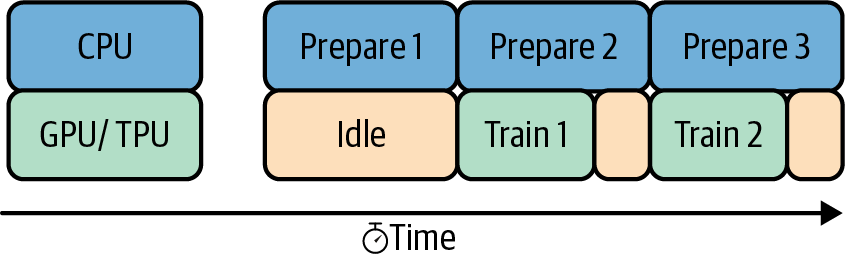
As GPUs can perform arithmetic operations much faster than CPUs, we see more model training use GPU for speed up. However, one still needs CPUs to process other tasks that involve disk I/O. If not handled properly, the CPU tasks can become the bottleneck and diminish the benefit brought by GPUs and Distribution Strategy. A simple optimization is to overlap the CPU and GPU tasks, such as using the TensorFlow tf.data.Dataset.prefetch API (shown below).

Hyperparameter Tuning

Aside from data munging, hyperparameter tuning is arguably where an ML practitioner spends most effort on. This design pattern aims to help us to do it better.

Grid search

This is the most common approach one would take: one simply iterates through the combinations of a set of hyperparameter ranges. As straightforward as it is, the combinatorial explosion will kick in fairly quickly. This is particularly an issue for large models where a single training run can take hours or days.

Instead of meticulously trying every single hyperparameter combination, one could specify the total number of trials, and then for each trial, one randomly chooses a new hyperparameter combination. This would bound the hyperparameter turning budget, but not necessarily bringing us the best outcome.

Bayesian optimization

Bayesian optimization is a technique for optimizing black-box functions. In this case, we can conveniently consider the hyperparameter values as the input to the black-box function, and the loss of the ML model as the output of this black-box function. A simple example to illustrate the general concept of Bayesian optimization is: if we have observed that increasing the max_depth of our xgboost model has not led to reduction of error metrics, then we probably won’t keep exploring deeper trees.

There is another layer of optimization added to the process. Bayesian optimization defines a new function that emulates our model but is much cheaper to run. This is referred to as the surrogate function. Again, the inputs to this function are hyperparameter values and the output is the optimization metric (e.g., loss).

I found this video a good introduction to Bayesian optimization (and the corresponding tutorial), and will probably learn more about it in the future.