Notes on Reinforcement Learning: MDP

In the previous note, we have highlighted the difference between Bandit and Reinforcement Learning (RL). In the former, the reward is immediate, and we want to identify the best action that maximizes this reward. In the latter, the reward is usually delayed, and the best action depends on the state where the agent is in. Moreover, the action will impact the future reward, so any action will have long term consequences.

This process can be modeled as Markov Decision Process, MDP. The central assumption of MDP is the memoryless Markov property: given the current state \(s\) and action \(a\), the both the state transition probability and the reward probability are independent of all previous states and actions. If both the state space and action space are finite, then it is called a finite MDP.

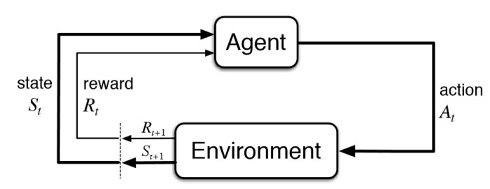
The diagram below illustrates the close-loop nature of a RL system: the agent interacts with the environment by taking actions, receiving rewards, and moving to a different state.

Nomenclature

We have introduced some nomenclature in the previous post, mostly in the context of bandit. Here we will add the common terminologies used in the RL context. Similarly, the subscript \(t\) denotes the time step.

Symbol	Definition
\(\pi(a\mid s)\)	An policy, which in general is probability distribution. It prescribes the probability of taking action \(a\) in the state \(s\).
\(v_\pi (s)\)	The state-value function of state \(s\), under the policy \(\pi\).
\(q_\pi (s, a)\)	The action-value function of state-action pair \((s, a)\), under the policy \(\pi\).
\(p(s', r \mid s, a)\)	The joint probability distribution of transition and reward.
\(G_t\)	Total rewards from time step \(t\), i.e., including future rewards.
\(\gamma\)	Discount rate of future rewards.

Policy

A policy \(\pi\) defines the action, \(a\), the agent will take, when in a given state, \(s\). The policy can be either deterministic (for example: when seeing a 4-way roundabout, alway turn left), or probabilistic (for example: 50% chance turn left, 15% chance go straight, 15% chance turn right, 20% chance turn back). After taken each action, the agent will receive a reward, \(r\), from the environment. This reward is usually stochastic as well.

The goal of RL is to find a policy that maximizes the total reward in the long term.

Value functions

For a given policy, one can calculate the value function: it estimates the future return under this policy. There are two types of value functions: state-value function, and action-value function. They are defined as:

\[\begin{align} v_{\pi}(s) &= \mathbb{E}_{\pi}[G_t | S_t = s]\\ q_{\pi}(s, a) &= \mathbb{E}_{\pi}[G_t | S_t = s, A_t = a] \end{align}\]

Note here \(G_t\) is the total reward from time step \(t\), that is, it is the sum of \(R_{t + 1}, R_{t + 2}, ...\), until the episode stops (e.g., winning a chess game), or into infinity.

To make it tractable, in the case of non-episodic process, the concept of discounting is introduced. In this setting, the future rewards are discounted, and \(G_t\) is now defined as:

\[G_t := R_{t + 1} + \gamma R_{t + 2} + \gamma^2 R_{t + 3} + ... = R_{t + 1} + \gamma G_{t + 1}\]

Obviously the discount rate \(\gamma \in [0, 1)\). Specifically, if \(\gamma = 0\), then we only consider the immediate reward, hence turning into the bandit case.

Intuitively, the value function measures how good it is to be in a given state (or taking a given action in a given state). For example, in a 2-dimensional grid world, if the goal is to reach a certain cell, then cells (states) close to the goal cell would have a higher state-value (assuming taking less moves are desired). Also, the value functions depend on the policy \(\pi\): in this grid world example, if the policy prescribes the agent to always move left, then the state left to the goal-state will have a state-value function smaller than that of a policy to always move right.

The goal of RL can then be boiled down to:

1. How to calculate the value functions for a given policy.
2. How to find the policy that has the highest value functions.

Dynamic programming and Bellman equation

For a given policy \(\pi\), if the transition probability \(p(s', r \mid s, a)\) is known, then the a single state-value function can be described by other state-value functions as:

\[\begin{align*} v_{\pi}(s) &= \sum_{a} \pi(a | s) \sum_{s', r} p(s', r \mid s, a)\big[r + \gamma ~ {\color{red} v_{\pi}(s')}\big] \\ &\text{for all } s \in \mathcal{S} \end{align*}\]

Intuitively, it states that the value of the given state, \(v_\pi(s)\), consists of the immediate reward, \(r\) and the discounted state-values of all possible successive states, \(v_\pi(s')\). It also depends on what action does the agent take – controlled by \(\pi\), and what is the future state – controlled by \(p(s', r \mid s, a)\).

Note that, the state-value function of \(v_\pi(s)\) is expressed recursively (its own value included on the right-hand side), as if we know all state-value functions \(v_\pi(s')\). This is the hallmark of dynamic programming. In this RL setting, this is known as the Bellman equation.

For a given RL problem, there are \(\mid \mathcal{S} \mid\) state-value functions, one for each state. Therefore, it is a set of linear equations, and in principle, can be solved analytically. However, it is usually infeasible to do so in practice, since the number of states is too large. Later we will introduce iterative algorithms to solve for the value functions.

The Bellman equation answers the question of “how to calculate the value functions for a given policy”

Similarly, one can derive the Bellman equation for the action-value functions as:

\[\begin{align} q_{\pi}(s, a) &= \sum_{s', r} p(s', r | s, a)\big[r + \gamma ~ \sum_{a'} \pi(a' | s') {\color{red} q_{\pi}(s', a')}\big]\\ &\text{for all }s \in \mathcal{S}, a \in \mathcal{A} \end{align}\]

There are \(\mid \mathcal{S} \mid \times \mid \mathcal{A} \mid\) action-value functions. Note that the second summation (over \(a'\)) amounts to \(v_{\pi}(s')\).

To answer the second question we posted above, namely, how to find the that has the highest value functions, we will leave it to the next post.

Markov Reward Process

In the preceding discussion, there is a policy embedded in the process (hence a decision process). If we remove this component, such that the system will transition between different states following its own (stochastic) dynamics, but still allow the agent to collect rewards at each state, we reduce the MDP to the Markov Reward Process (MRP).

One can still write the Bellman equation for state value functions in the case of MRP, but in a simpler way. Without consideration of taking actions, and associate the reward to the target state \(s'\), the transition probability becomes \(p(s' \mid s)\), and the Bellman equation is:

\[\begin{eqnarray} v(s) = \sum_{s'}p(s' \mid s)[r(s') + \gamma {\color{red} v(s')}]. \end{eqnarray}\]

This is still a linear system of equations, but can expressed in a compact matrix notation as:

\[V = P (R + \gamma V),\]

where:

\[\begin{eqnarray} V &=& \begin{bmatrix} v(s_1) \\ v(s_2) \\ ... \\ v(s_N) \end{bmatrix}, \\ P &=& \begin{bmatrix} p(s_1 \mid s_1) & p(s_2 \mid s_1) & ... & p(s_N \mid s_1) \\ p(s_1 \mid s_2) & p(s_2 \mid s_2) & ... & p(s_N \mid s_2) \\ \vdots & \vdots & \ddots & \vdots \\ p(s_1 \mid s_N) & p(s_2 \mid s_N) & ... & p(s_N \mid s_N) \end{bmatrix}, \\ R &=& \begin{bmatrix} r(s_1) \\ r(s_2) \\ ... \\ r(s_N) \end{bmatrix}. \end{eqnarray}\]

Therefore, the solution for the value function is:

\[V = (I - \gamma P)^{-1} PR\]

assuming \((I - \gamma P)\) is invertible.