Notes on Reinforcement Learning: Policy and value iterations

We will limit the following discussion in the case of deterministic policy.

Policy evaluation (prediction)

In the previous post, we described the Bellman equation as the foundation to solve for the (state- or action-) value function under a given policy. We further argue that, despite its closed-form nature, it is infeasible to solve it analytically. In practice, we use an iterative algorithm called dynamic programming (DP).

Simply put, for the policy \(\pi\) under evaluation, we first initialize the state value function with some random values (e.g., all zeros). Next, we will start the main loop. In each iteration of the main loop, we will update each of the value functions \(v_{\pi}(s)\) using the Bellman equation:

\[\begin{align*} v_{\pi}(s)_{k+1} &\leftarrow \sum_{a} \pi(a | s) \sum_{s', r} p(s', r \mid s, a) \big[r + \gamma ~ {\color{red} v_{\pi}(s')_{k}}\big] \\ &\text{for all } s \in \mathcal{S} \end{align*}\]

Note that, when updating the value function for the \((k+1)^\text{th}\) iteration, the value functions used in the right-hand side of the Bellman equation take the value from the previous (i.e., \(k^\text{th}\)) iteration (so-called synchronous update). If the changes in value functions from consecutive updates are less than a pre-set threshold, we will consider it converged and exit the main loop.

Here we only consider the state-value functions, but the same iterative procedure can be applied to calculate the action-value functions, using the corresponding Bellman equation. The only difference is that, in each iteration, instead of \(\mid \mathcal{S} \mid\) state-value functions to update, now we have \(\mid \mathcal{S} \times \mathcal{A} \mid\) action-value functions to update.

This process, policy evaluation (a.k.a, prediction), is the task to determine the state-value function, \(v_\pi(s)\), for a given policy \(\pi\).

Optimal policy

Now we can evaluate the (state- or action-) value function of any policy, if the state-value function under a given policy is higher than under any other policy, then this state-value function is called the optimal state-value (subscripted with \(*\)), and the corresponding policy is called optimal policy, \(\pi_*\). Put differently, under the optimal policy, the corresponding value function at each state is the largest among all possible value functions. While the \(v_*(s)\) is unique (as they are scalar), there can be multiple optimal policies.

If we already know the optimal state-value functions, \(v_*(s)\), it is quite trivial to find the optimal policy, as:

\[\pi_*(a \mid s) = \text{argmax}_{a} \sum_{s', r}p(s', r \mid s, a)\big[r + \gamma v_*(s')\big]\]

Basically, at each state \(s\), we choose the action that maximizes the expected total future rewards. Along this line of logic, one can reason the form of the Bellman optimality equation as (note that no policy is involved):

\[\begin{align} v_{*}(s) &= {\color{red}{\max_{a}}} \sum_{s', r} p(s', r \mid s, a)\big[r + \gamma ~ {v_{*}(s')}\big] \\ q_{*}(s, a) &= \sum_{s', r} p(s', r | s, a)\big[r + \gamma ~ {\color{red}{\max_{a'}}}~{q_{*}(s', a')}\big] \end{align}\]

If the state-value function for a given policy – calculated by the generic Bellman equation – equals the state-value function derived from the Bellman optimality equation, then this policy is the optimal policy, \(\pi_*\), and the state-value function is accordingly called \(v_*\). Note that \(v_*\) is unique, but there can be multiple \(\pi_*\) lead to the same \(v_*\).

Policy improvement (control)

Given the link between the optimal value and optimal policy, and the fact that the ultimate goal of reinforcement learning is to find the optimal policy, we need to devise an algorithm to improve the policy. This process, policy improvement (a.k.a, control), is the task to improve the policy towards the optimal policy.

There is a greedy way to improve a given policy. From the policy evaluation, one obtains the all the state-value functions. From here, there is a way to achieve an equally good, or better policy, by taking greedy action at each state. Simply put, if the current policy \(\pi\) instructs an action at the given state \(s\), then a new policy \(\pi'\) subscribes that:

\[\begin{align*} \pi'(s) = \text{argmax}_{a}\sum_{s', r}p(s', r \mid s, a)[r + \gamma v_\pi(s')]. \end{align*}\]

Note the state-values are still under the current policy \(\pi\).

Alternatively, if we use the action-value function, the greedy policy improvement becomes simpler: for a given state, the new policy will pick the action with the highest action-value function.

Policy iteration

With the policy evaluation and policy improvement in place, we can see there is a clear link between them. Furthermore, it is not hard to see the iterative nature. This is the so-called policy iteration algorithm, in order to find the optimal policy.

Starting from a random policy, we will iteratively:

• With the current policy, apply policy evaluation, to update the value function.
• With the current value function, apply policy improvement, to update the policy.

This process exits if the policy stops changing.

Note that, a single policy evaluation step itself is also an iterative process, which only terminates after an exit condition is met, i.e., the value-function stops changes between successive iterations.

General policy iteration and value iteration

The policy iteration algorithm has a nested iterative nature: the policy update itself is an iterative process, whereas in each of the policy updates, we need to evaluate the state-value functions for the given policy, which itself is an iterative process. This can be computationally expensive, and yet with a slight change, we can avoid such a nested structure. This is where the value iteration algorithm comes in.

The value iteration algorithm side-step the policy evaluation step altogether: instead of finding the state-values for the given policy (run the iterative policy evaluation step until convergence), it tries to find the optimal state-values directly. This is achieved by greedily selecting the action that maximizes the state-value, i.e., without following any policy. This is done with the Bellman optimality equation:

\[\begin{eqnarray} v_{k+1} (s) \leftarrow \max_{a} \sum_{s', r}p(s', r \mid s, a)[r + \gamma v_{k}(s')] \end{eqnarray}\]

Effectively, we use the Bellman optimality equation as the update rule, to iteratively solve for the optimal state-value functions. Once the optimal state-value functions are obtained, we simply greedily select the action, to arrive at the optimal policy.

Note that in this algorithm, there is no policy involved when calculating the state-value functions, hence the name value iteration.

More generally, the dance between updating the value function, and updating the policy consists path to the optimal value function \(v_*\) and optimal policy \(\pi_*\). The picture below illustrates this process: an arrow that goes toward the “value” line indicates a policy evaluation (prediction) step, and an arrow that goes toward the “policy” line indicates a policy improvement (control) step.

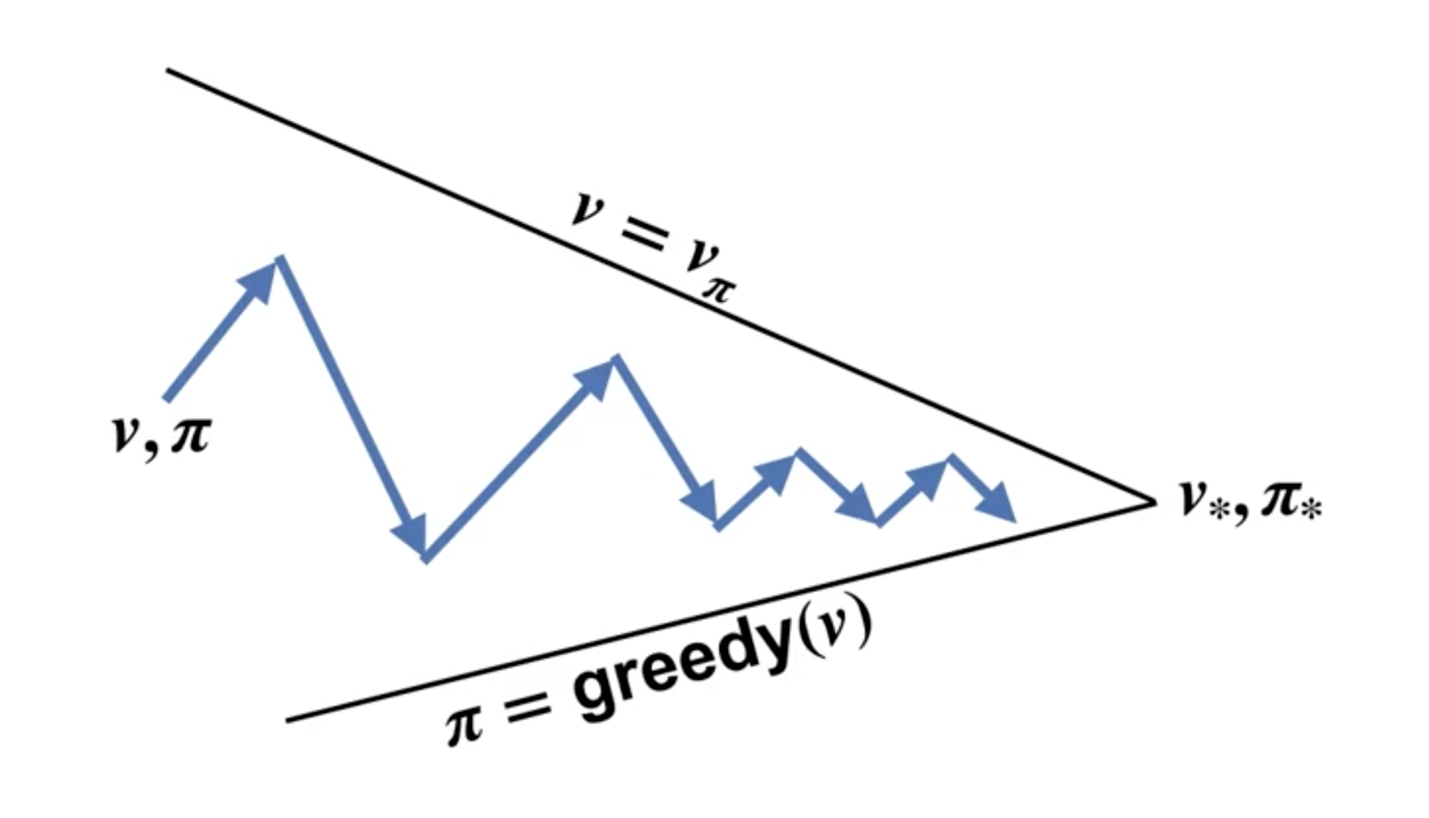
For the policy iteration algorithm, the arrow will touch each line, indicating a converged iteration, however, for a general policy iteration (e.g., value iteration), we can lose the requirements and still find the ultimate convergence.