Notes on Reinforcement Learning: Monte Carlo method

Found another good course from Stanford (video recordings from winter 2019). If the official site is not working, this Github repo contains most of the materials.

In the previous notes, we laid out the foundation of reinforcement learning (RL), and most importantly, the concept of MDP, state, reward, policy, state value, (state-)action value, and how to find the optimal policy that leads to the largest state values. However, all the calculation are based on the assumption that there is a model that dictates the transition probability between different states, namely, \(p(s', r \mid s, a)\). It is not hard to see, this assumption (that we have the complete knowledge of the environment) can be easily violated. The Monte Carlo (MC) method helps us to move from a model-based situation to a model-free situation.

Monte Carlo method

In the model-based paradigm, we use the Dynamic Programming (DP) method to iteratively calculate the state values \(v(s)\). To find the optimal state value \(v_{*}(s)\), we can use either policy iteration, or value iteration. Once \(v_{*}(s)\) is found, we can use the \(\text{argmax}\) to greedily find the optimal policy \(\pi_{*}\).

The essence is to find a good estimate of \(v_{\pi}(s)\). If there isn’t a model for use to apply the DP method, in the episodic case, we can use sample average as the estimate of \(v_{\pi}(s)\), from multiple episodes following the same policy \(\pi\). This is what MC method entails.

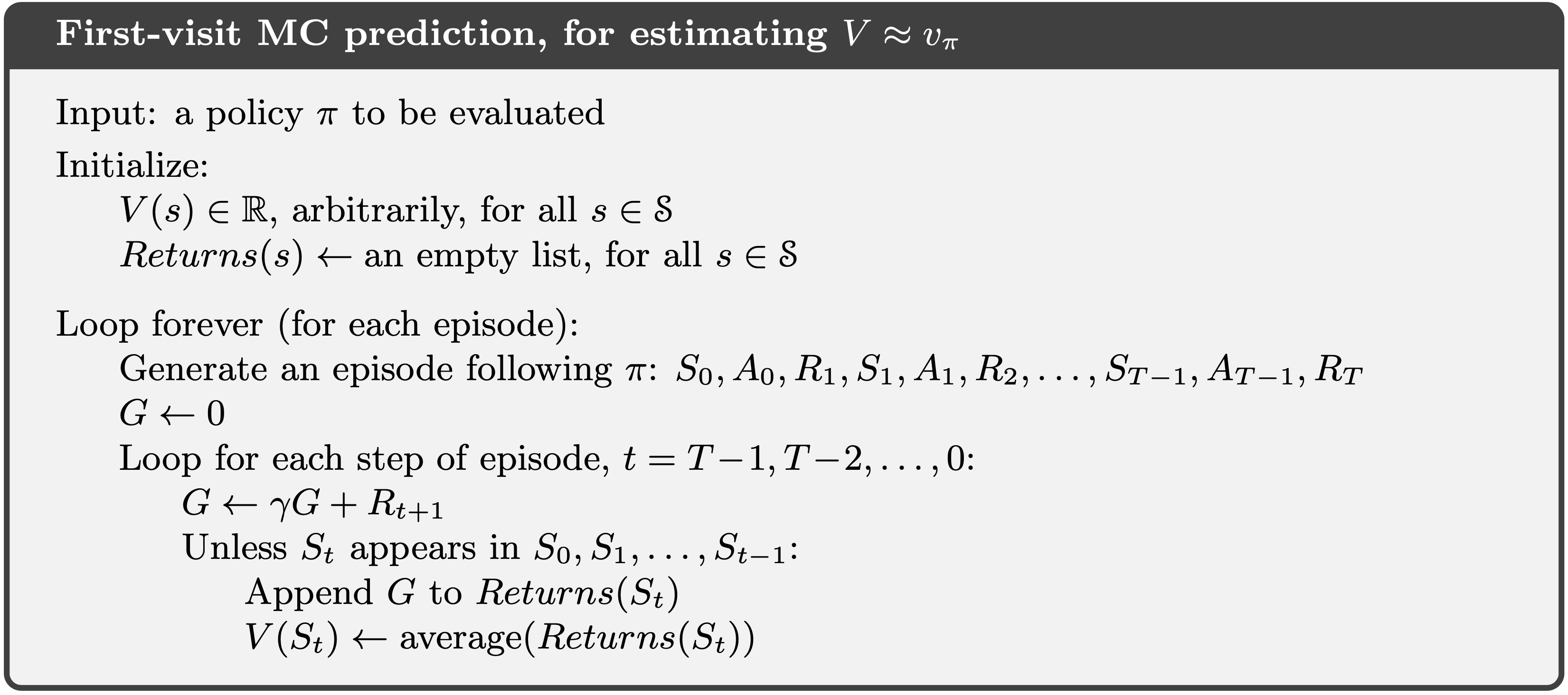
In the context of episodic tasks (with terminal states), after an episode (1, …, \(t\), …, \(T\)) is finished (following the policy \(\pi\)) and total rewards \(G_T\) collected, we can count from the back (\(T\)), and calculate the discounted rewards \(G_t\) of each of the passing states \(s_t\). As such, we are sampling \(v_\pi(s)\) from the episode, and from the definition of the state value function (note the expectation notation), we can use sample average as the estimation for the true \(v_\pi(s)\). Note that, for the same episode, the same state \(s\) can appear more than once.

We can run through many episodes, in the hope to visit each state multiple times, and the state values can be estimated as the simple average. The same procedure can be used to estimate the state-action values.

First visit and every visit

As mentioned above, the same state can be visited multiple times during the same episode, and it matters which visit (or all) should be used in the sample averaging. Being an estimator, we need to discuss its bias and variance. It turns out that, if we limit ourselves in the first visit (of the multiple visits to the same state) in a single episode, it is a unbiased estimator. If we use every visit to the same state in a single episode, it would lead to a biased estimator (think the following visits are correlated from the initial state). However, the every visit estimator is more data efficient as we don’t discard the following visits.

Another aspect to consider is how to ensure exploration in MC? Exploring start (similar to the optimistic initial values in bandit) can help to address this, by randomize the initial state. In the following states, the agent will follow the prescribed policy. There are certain limitations of exploring start though, maybe it is not feasible in reality. We can do better: taking a page from the \(\epsilon\)-greedy policy in the multi-armed bandit setting: when deciding which action to take in the episode, instead of deterministically follow the current policy \(\pi\), there is a small probability, e.g., \(\epsilon\), the agent will choose a random action.

Incremental update

Since the estimation of state value is taken as the sample average, with more data coming in, the update rule can be written as:

\[v_{k + 1}(s) = v_k(s) + \alpha (G_i(s) - v_k(s))\]

Here, \(i\) indicates the newly observed total reward from state \(s\), from episode \(i\) (we use the first visit algorithm here), \(k\) indicates the index of the update iteration, and \(\alpha\) can be thought as the learning rate: when it is set to \(1 / N(s)\), where \(N(s)\) is the total number of visits to state \(s\), the above formulation returns to the simple sample average. However, when written as such, it is:

• More space efficient: we don’t need to maintain the full history of \(v(s)\) as an array, but only the most recent one, and \(\alpha\).
• More flexible to accommodate other update rules, for example, a constant value, to place more weight on recent observations.

Another benefit is that, such an incremental update formulation will lead us naturally to the next topic: temporal difference learning.

Comparison to Dynamic Programming (DP)

As mentioned in the beginning, the biggest advantage of MC over DP is that, in MC, we don’t require to know the model that prescribes the transition dynamics. Instead, we directly use the experience from interacting with the environment to incrementally update the estimation of the state values. Even in the situation where it is possible to obtain the transition dynamics, it can be tedious and error-prone, therefore MC can be preferred over DP. Moreover, when updating the state value \(v(s)\), we don’t rely on the estimates of other state values \(v(s')\), namely, we do not bootstrap.