Notes on Reinforcement Learning: Temporal Difference learning for prediction

The Monte Carlo (MC) method for (state) value function estimation is an approach that does not rely on a model to predict the system dynamics, namely, the probability of state transition and reward under a given action. This is more practical as in real world, it is unlikely that we can have the full understanding of the system, to allow us writing down the \(P(s', r \mid s, a)\).

Temporal Difference (TD) learning is another model-free framework, that combines the characteristics of MC and the model-based Dynamic Programming (DP) method. It also address the drawback in MC that it only applies to the episodic situation.

TD for prediction

So far, the central theme of reinforcement learning is to solve for, or estimate the value functions, be it state values or state-action values (prediction problem). In DP, we leverage the concept of bootstrap: when investigating a single state, we assume we already know the values for other state values, and construct the Bellman equations to solve for it. In MC, we allow the agent to take actions and experience the environment (sampling). As the agent visits different states and collecting rewards, we do careful bookkeeping and then update the state values retrospectively, after an episode is terminated.

TD combines the concept of bootstrap from DP, and sampling from MC. With TD method, the agent also interacts with the environment by taking actions. However, once the agent transitioned from state \(s_t\) to \(s_{t + 1}\), and collecting the reward \(r_t\), it will update the state value \(V(s_t)\) as:

\[V(s_t) \leftarrow V(s_t) + \alpha \overbrace{(\underbrace{[r_t + \gamma V(s_{t + 1})]}_{\text{TD target}} - V(s_t))}^{\text{TD error}},\]

where \(\alpha\) is a newly introduced variable dubbed as learning rate.

Conceptually, we make correction to the current estimate of the state value, with a “TD error” term multiplied the learning rate. Inside the construct of the TD error, the term “TD target” can be viewed as the estimation of true \(V(s_t)\), as if we know the true value of \(V(s_{t + 1})\) (based on the definition of the state value). This assumption is the very nature of bootstrap.

Note that, like DP, TD bootstraps, but unlike DP, TD does not require a model. Like MC, TD samples the environment to update the value functions, but unlike MC, TD does not need to wait for the end of an episode to update the state values: TD makes updates immediately after every action. In a way, TD takes the best of the two worlds.

A simple example

Let’s use a simple example to demonstrate how these 3 methods work in estimating the state values.

In this example (Barto and Sutton, Example 6.2), the agent starts from state 3, and always takes a 50/50 chance between moving left or right. The state 0 and 6 are terminal states, and moving from state 5 to 6 gives the agent a reward of +1, all other transitions have no reward. As such, this is an episodic task. We will use DP, MC and TD to solve for the state values. (Jupyter notebook here)

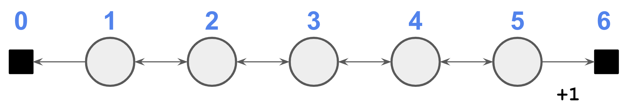
For the sake of simplicity, the discount factor \(\gamma\) is set to 1.

Dynamic Programming (DP)

To use DP, we need to write down the state transition probability \(P\), along with the rewards probability \(R\). Using a matrix notation, they can be written as:

\[\begin{eqnarray} P &=& p(s' \mid s) = 0.5 \times \begin{bmatrix} 0 & 0 & 0 & 0 & 0 & 0 & 0 \\ 1 & 0 & 1 & 0 & 0 & 0 & 0 \\ 0 & 1 & 0 & 1 & 0 & 0 & 0 \\ 0 & 0 & 1 & 0 & 1 & 0 & 0 \\ 0 & 0 & 0 & 1 & 0 & 1 & 0 \\ 0 & 0 & 0 & 0 & 1 & 0 & 1 \\ 0 & 0 & 0 & 0 & 0 & 0 & 0 \end{bmatrix} \\ R &=& \begin{bmatrix} 0 & 0 & 0 & 0 & 0 & 0.5 & 0 \end{bmatrix} \end{eqnarray}\]

The indices in \(P\) and \(R\) correspond to the state indices. The state values \(V\), also written in a matrix notation, can then be solved via Bellman equation as:

\[\begin{eqnarray} V &=& P(R + \gamma V) \\ &\Downarrow& \\ V &=& (I - \gamma P)^{-1} P R \end{eqnarray}\]

The state values turn out to be:

\[V = [0, \frac{1}{6}, \frac{1}{3}, \frac{1}{2}, \frac{2}{3}, \frac{5}{6}, 0]\]

Note this will be used as the ground truth against which the MC and TD methods will compare.

Monte Carlo (MC)

To apply MC, we will run a series of simulations. In each episode, the agent will start from state 3, and terminate at either state 0 or 6. Once an episode is terminated, we will update the state value of visited states from the back. Here we will use the first visit MC.

Temporal Difference (TD)

In TD, we also run a series a simulations, starting from state 3. However, as soon as transition from an old state to a new state, we apply the updating rule outlined above, to arrive at a new estimation of the state value of the old state.

Comparisons

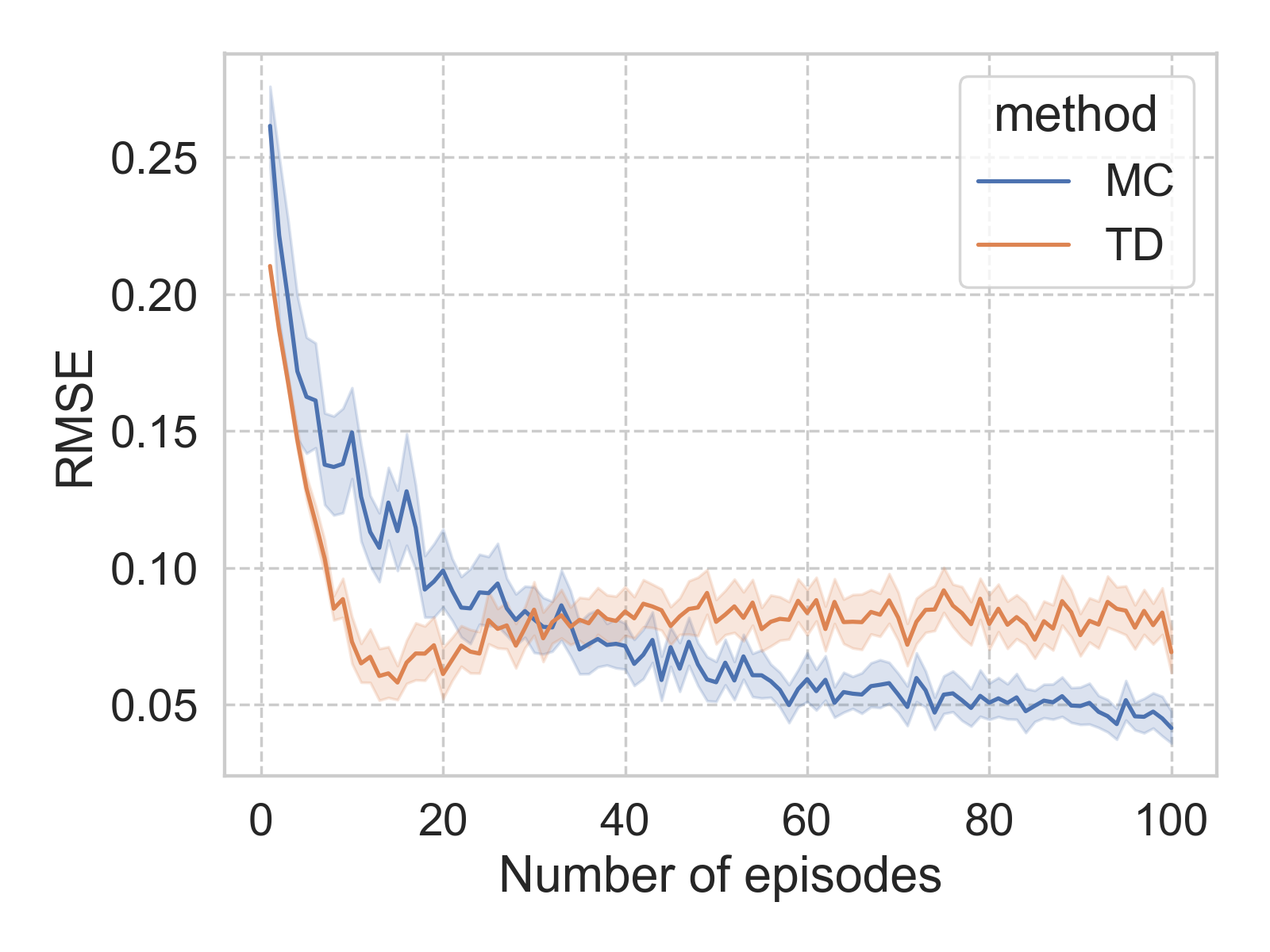
With 100 episodes, both the MC and TD methods arrive at a reasonably well estimate of the state values (quantified by the RMSE). It is also clear that, with more episodes, both the MC and TD methods are achieving better results (smaller RMSE), albeit with different rates, and seemingly different asymptotic limit. However, it is worth noting that both the convergence rate and limit are impacted by the hyperparameter of the model, such as learning rate.

Conclusion

Here we discussed TD as the second model-free method to estimate the state value functions, and this is in the larger context of policy evaluation (prediction) framework. More specifically, the method is TD(0) (we will see a more general TD(\(\lambda\)) algorithm later). Compared to MC, TD usually converges faster, and it is truly incremental and online.