Gradient descent with the right step

The central theme for many machine learning task is to minimize (or maximize) some objective function \(f(\theta)\), often consists of a loss term and a regularization term. Well, how hard is it to find the minimum value for \(f(\theta)\)? Just get the first derivate, i.e., gradient, \(\nabla f(\theta)\), set it to zero, and solve for the magical \(\theta_\text{magical}\) such that \(\nabla f(\theta_\text{magical}) = 0\), problem solved! (Let’s assume there is indeed a global minimum…) Only can it be so easy. In many (if not most) cases, there is no analytical solution for \(\nabla f(\theta) = 0\), therefore we want to use some other means to find the minimum of \(f(\theta)\), and gradient descent is our best choice.

How does gradient descent work

Recall Taylor expansion for our \(f(\theta)\), at a given location \(\theta_0\):

\[\begin{eqnarray} f(\theta) = f(\theta_0) ~+~ \nabla f(\theta_0) \Delta \theta ~+~ ..., \end{eqnarray}\]

where \(\Delta \theta = \theta - \theta_0\). If we already know the value of \(\theta_0\), hence \(f(\theta_0)\), what value of \(\Delta \theta\) I should use, such that I can be almost sure that \(f(\theta_0 + \Delta \theta)\) will be smaller than \(f(\theta_0)\)? If I can always achieve this goal, at any \(\theta\), then I will get to the minimum of \(f(\theta)\). Staring at the Taylor expansion, you can easily find that, if I set \(\Delta \theta\) to \(-\nabla f(\theta_0)\), or \(-\eta \nabla f(\theta_0)\) with \(\eta > 0\), then I will have:

\[\begin{eqnarray} f(\theta_0 + \Delta \theta) = f(\theta_0) ~-~ \eta (\nabla f(\theta_0))^2 ~+~ .... \end{eqnarray}\]

If I just ignore the higher order terms, then I got what I wanted: \(f(\theta_0 + \Delta \theta)\) will be smaller than \(f(\theta_0)\). The key is to find the right \(\Delta \theta\): clearly, \(\nabla f(\theta_0)\) is the gradient at \(\theta_0\), and the parameter \(\eta\) is usually called step size, or learning rate. Putting these two terms together: \(\nabla f(\theta_0)\) gives me the direction for the next step, and \(\eta\) gives me the size of the step. The pseudo code is as simple as:

# gradient descent
for i in range(max_epoch):
    gradient = gradient_fn(param, data)
    param -= step_size * gradient
    if converge:
        break

In addition, we can track the values of \(f(\theta)\) at each step, just to make sure it does decay monotonically. Note that, the objective function (and its gradient) usually takes data as input as well, namely, \(f(\theta) = f(\theta; X)\), and \(\nabla f(\theta) = \nabla f(\theta; X)\).

There you have it: gradient descent can be clearly understood through the lens of Taylor expansion. But remember that our first order Taylor expansion is only valid in the neighborhoods of its expansion loci, therefore if the step size is not chosen properly, namely, if the step size is too large, then all our previous derivation will go down the drain. Then, how large is too large?

Let’s go through an example to drive the point home. Say we have \(f(\theta) = (\theta - 5)^2\). It is clear that \(\theta_\text{magical}\) = 5, with \(f(\theta_\text{magical})\) = 0 as its minimum. If I insist to use gradient descent, how should I do it? Simple enough, we have \(\nabla f(\theta) = 2(\theta - 5)\), the only other thing I need is to choose a proper step size. Hmmm, how about 0.1? It turns out 0.1 works just fine, as you can find below. The codes can be found here.

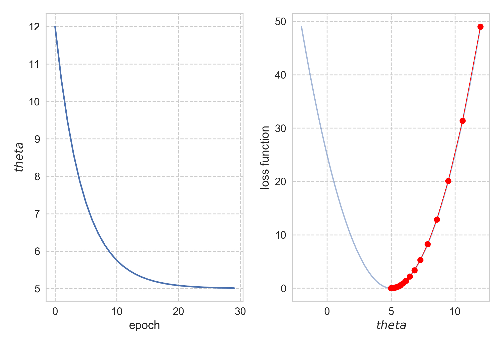
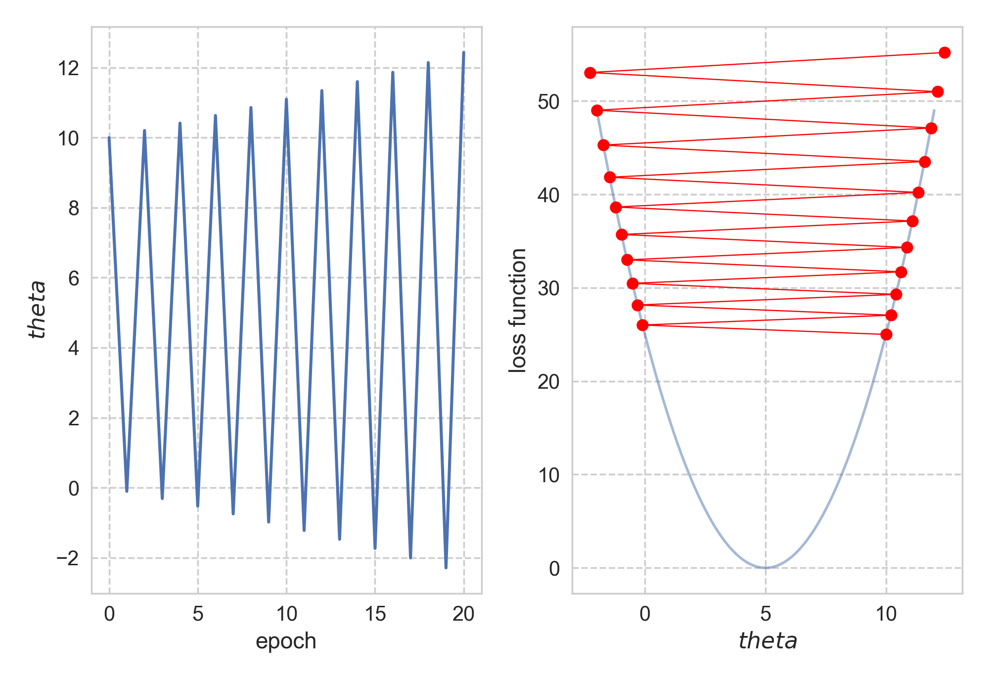
Starting from \(\theta_0\) = 12, it took us 29 steps to reach convergence. What if I want to get to the bottom faster, i.e. with fewer steps? Naturally, I would just increase the step size: let’s do 1.01 instead of 0.1! The same procedure now turns against me, as starting from 10, \(\theta\) swings away from 5.

Backtracking line search

So too big a step size is disastrous, too small a step size will cause us time, how to find the right step size, for each iteration? Here comes the idea of backtracking line search. The idea is rather simple: at each iteration, before we decide a step size, let me try some really large one, and (this is the key) to see whether with this step size (and the resulting \(\Delta \theta\), we can make the objective function smaller, i.e. \(f(\theta + \Delta \theta) < f(\theta)\), and if (1) is satisfied, then (2) make it decrease by a certain amount. If not, then don’t use this step size, but shrink it a little bit, say, by half, and test the new, smaller step size again.

# backtracking line search
for i in range(max_iteration):
    current_loss = loss_fn(param)
    new_param = param - step_size * gradient_fn(param)
    new_loss = loss_fn(new_param)
    if not new_loss - current_loss < threshold:
        step_size *= 0.5
    else:
        break
return step_size

In the pseudo code above, the threshold will be set differently at each \(\theta\). Essentially, we are doing another lousy optimization to find the “good enough” step size: we don’t really want to spend too much computation just to find the best step size. Compared to the previous “one-size-fits-all” step size, here we are changing the step size adaptively. For more rigorous derivations, here is a good reference.

Then how does this simple idea work in practice? Well, it works pretty well. Below you can find the optimization path for the aforementioned one-dimensional case, it is quite obvious that we like to use backtracking line search for sure.

Just for fun, let’s try somewhat slightly “harder” case, to fit a univariate Gaussian distribution. There are two scalar values to be fitted: mean and variance, hence this can be considered as a two-dimensional case. The script can be found here. Again, the backtracking line search gets us to the minima with fewer steps, as shown below. The scale bar indicates the values of the loss function (negative of the log likelihood).

There are much more

The purpose of the backtracking line search is to find the appropriate step size, or at a higher level, the appropriate \(\Delta \theta\) for the next parameter update. It is clear one needs to adaptively make the update, and backtracking line search is just one of the strategies. It can be argued that backtracking line search can be computationally expensive, given the iterative steps we spend on searching for single step size, especially for large datasets: simply evaluating the loss function or gradient can take a while. There are better methods to pick \(\Delta \theta\), such as using momentum (remember previous \(\Delta \theta\) s) while updating \(\theta\). For the curious minds, here is a rather comprehensive summary of the popular gradient descent algorithms.

In the end, it is all about finding the right step.