Spectral clustering, step by step

I was drawn to this problem from a colleague’s project: he needs to cluster some hundreds of thousands of distributions. There are two steps in this process: first, one needs to define how to properly measure the similarity (or equivalently, distance) between two distributions, and second, how to perform the clustering. For the former, a modified, symmetric Kullback–Leibler divergence is used, whereas for the latter, he uses spectral clustering. Priding myself on knowing a thing or two about spectral analysis from the academic days, I was like, spectral what?

The spectrum where Time is involved

Let me start with the spectral analysis that I was familiar with. Usually it takes some time series data as the input, and convert this time-domain signal to a different representation in the frequency domain. Experimentally, the time-domain to frequency-domain conversion is usually carried out numerically by fast Fourier transform (FFT). If one has the fortunate to afford a spectral analyzer, the conversion can be performed with hardware, for example, by superheterodyne down-mixing.

It works best with an example. Think a frictionless pendulum: we can either describe its steady-state motion by its angle \(\theta(t)\), whose value changes with time \(t\), or simply describe the essence of the pendulum with its oscillation period (or frequency) and amplitude, which are fixed values. Both the time-domain and frequency-domain representations carry the same information, but apparently the frequency-domain representation is more concise. Scaling up from this simple case, one can easily learn more about the underlying system by observing characteristics from the frequency spectrum. This convenience highlights the benefits of spectral analysis, and it is why it has found itself enormously important in scientific research.

The spectrum where a graph is involved

Apparently, there is no Time involved in this clustering problem. Instead, here we want to group different data points into different clusters. It is best to think this problem in the context of a graph: each data point – be it a distribution, a person, or any abstract object – can be treated as a vertex of the graph. The similarity between any pair of data points can be viewed as the weight of the edge that connects the two vertices.

Note that here we need to have a clear definition of the similarity measure. In the most intuitive point-on-2D-plane example, where we can easily define the Euclidean distance, a Gaussian kernel can be applied to transform the distance measure to the corresponding similarity measure. Since the similarity measure is always valid for all pairs, the underlying graph is fully connected. One can also apply some constraints to make the graph sparse.

A natural way to represent a graph is using adjacency matrix. Since here we are dealing with an undirected graph with non-negative edge weights, the adjacency matrix is real and symmetrical. There is one problem though: how do we determine the diagonal elements of the matrix, namely, the similarity between a vertex and itself? It turns out that, for this problem it doesn’t really matter, and for convenience, let’s just assign them with 0. It will become clear why this is the case later.

An example will make things much clearer. Below is a simple graph with 6 vertice and 8 edges, with edge weight indicating the similarity between the connecting vertices. It is a little bit counter-intuitive since we are not considering (Euclidean) distance which is visually appealing, but rather the reverse, namely, similarity. Also, if there isn’t an edge between two vertices, we consider the similarity to be zero.

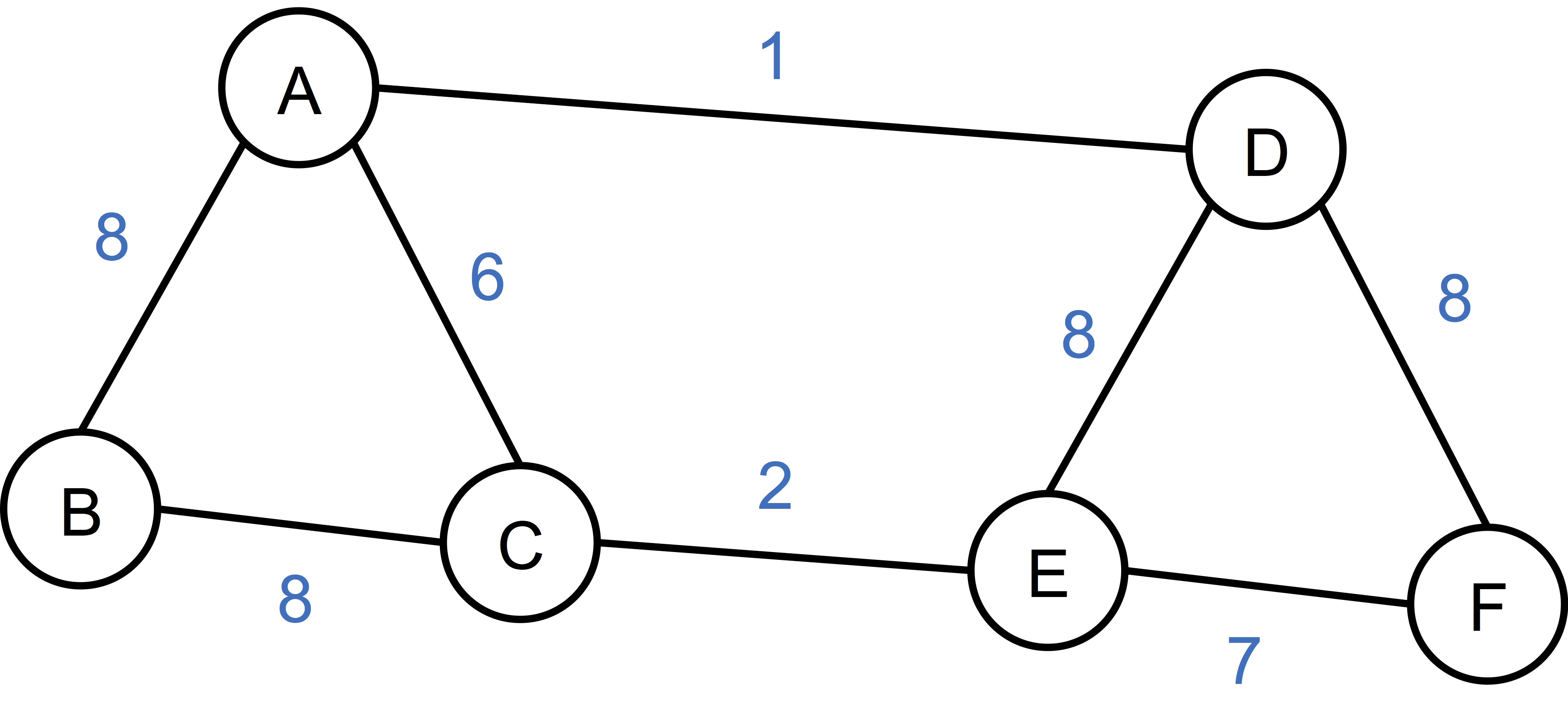
Let’s construct the adjacency matrix \(S\) real quick, as:

\[S = \begin{bmatrix} 0 & 8 & 6 & 1 & 0 & 0 \\ 8 & 0 & 8 & 0 & 0 & 0 \\ 6 & 8 & 0 & 0 & 2 & 0 \\ 1 & 0 & 0 & 0 & 8 & 8 \\ 0 & 0 & 2 & 8 & 0 & 7 \\ 0 & 0 & 0 & 8 & 7 & 0 \end{bmatrix}.\]

Here I implicitly order the vertices alphabetically. The matrix \(S\) is also often denoted as \(A\) or \(W\), to reflect that it is the adjacency matrix, or weight matrix. At this juncture, we successfully convert the data to a graph, and further the corresponding matrix representation. Here onwards, we are going to deal with the spectrum of a matrix representation of the underlying graph, that is, the matrix’s set of eigenvalues together with their multiplicities. In another word, we want to explore the spectrum of the graph.

Spectral clustering as an optimization problem

The minimum cut

Once in the graph land, the clustering problem can be viewed as a graph partition problem. In the simplest case, in which we want to group the data to just 2 clusters, we are effectively looking for a graph cut which partition all the vertices to two disjoint set of \(A\) and \(B\), such that the objective function \(\mathcal{L}\):

\[\begin{eqnarray} \mathcal{L}(A, B) = \sum_{i \in A,~ j \in B} s_{ij}\\ \end{eqnarray}\]

is minimized. In another word, we want to minimize the total weights of all edges that cross the frontier of the cut. This effectively turns the clustering problem to a minimum cut problem, where there are well-developed algorithms.

The normalized minimum cut

However, this minimal cut paradigm does not always work well in real clustering problems (see figure 1 of this paper for an example). Instead, one would rather minimize the following objective function:

\[\begin{eqnarray} \mathcal{L}_\text{norm}(A, B) = \sum_{i \in A,~ j \in B} s_{ij} {\large(}\frac{1}{\text{vol}(A)} + \frac{1}{\text{vol}(B)}{\large)}, \end{eqnarray}\]

where \(\text{vol}(A) = \sum_{i \in A} d_i\). Here \(d_i\) is the degree of vertex \(i\), and \(\text{vol}(A)\) can be viewed as a measure of the size of the cluster. This “normalized” version of the minimum cut problem will penalize cluster with small size, therefore achieving more balanced clusters. Unfortunately, this normalized minimum cut problem is NP-hard, and one has to resort to the approximate solutions.

Graph Laplacians

In order to solve for the normalized minimum cut problem, one needs to analyze the Laplacian matrix, \(L\), of the graph, as \(L = D - S\). Here \(D\) is a simple diagonal matrix, with \(d_{ii}\) equals the sum of \(i^\text{th}\) row of \(S\). It should become clear now why the values of the diagonal elements of \(S\) is irrelevant, since they get canceled out in \(L\). As a result, each of the row sums for \(L\) is zero. As the frequency spectrum of a frictionless pendulum can reveal the essence of the motion, the eigenvalues and eigenvectors of the graph Laplacian will guide us to uncover the basic properties of the graph.

The Laplacian matrix for the simple example above is then:

\[L = \begin{bmatrix} 15 & -8 & -6 & -1 & 0 & 0 \\ -8 & 16 & -8 & 0 & 0 & 0 \\ -6 & -8 & 16 & 0 & -2 & 0 \\ -1 & 0 & 0 & 17 & -8 & -8 \\ 0 & 0 & -2 & -8 & 17 & -7 \\ 0 & 0 & 0 & -8 & -7 & 15 \end{bmatrix}.\]

From here, things start to diverge, in three major directions. One can either proceed with the graph Laplacian as it is; or one can normalize \(L\), in two different ways, as:

\[\begin{eqnarray} L_\text{sym} &=& D^{-1/2} L D^{1/2},\\ L_\text{rw} &=& D^{-1} L, \end{eqnarray}\]

where the subscripts \(_\text{sym}\) and \(_\text{rw}\) mean symmetric and random walk, respectively. Depending on which graph Laplacian is used, the clustering algorithm differs slightly in the details. In the below, I will follow the algorithm proposed in Ng, Jordan, Weiss, by using \(L_\text{sym}\) to perform the clustering task.

Spectral clustering, step by step

After laying out all the notations, we are finally ready to carry out a \(k\)-group clustering with the following steps:

1. Obtain the graph Laplacian as \(L = D ~–~ S\);
2. Normalize the graph Laplacian as: \(L_\text{sym} = D^{-1/2} L D^{1/2}\);
3. Get eigenvalues and eigenvectors of \(L_\text{sym}\), with the ascending order of eigenvalues;
4. Take the first \(k\) eigenvectors, and to form a \(N \times k\) matrix \(U\);
5. Form a matrix \(T\) from \(U\) by normalizing the rows of \(U\) to norm 1.
6. Treat each row of \(T\) as a data point, run some simple clustering algorithm such as K-means, make cluster assignments (1 to \(k\));
7. The original problem will be given the same cluster assignment.

It is worthwhile to go back to the running example, and carry it through the steps. The calculated \(L_\text{sym}\) is:

\[L_\text{sym} = \begin{bmatrix} 0.130 & -0.069 & -0.051 & -0.008 & 0. & 0. \\ -0.069 & 0.137 & -0.068 & 0. & 0. & 0. \\ -0.051 & -0.068 & 0.137 & 0. & -0.017 & 0. \\ -0.008 & 0. & 0. & 0.145 & -0.068 & -0.068 \\ 0. & 0. & -0.017 & -0.068 & 0.145 & -0.060 \\ 0. & 0. & 0. & -0.068 & -0.060 & 0.130 \\ \end{bmatrix},\]

and the corresponding \(T\) (with \(k\) = 2) is:

\[T = \begin{bmatrix} 0.706 & -0.708 \\ 0.677 & -0.735 \\ 0.738 & -0.674 \\ 0.710 & 0.703 \\ 0.740 & 0.672 \\ 0.677 & 0.735 \\ \end{bmatrix}.\]

At this point, without running a formal clustering algorithm, we can easily eyeball that the first three rows (vertices A, B, C) are in a different group of the bottom three rows (vertices D, E, F).

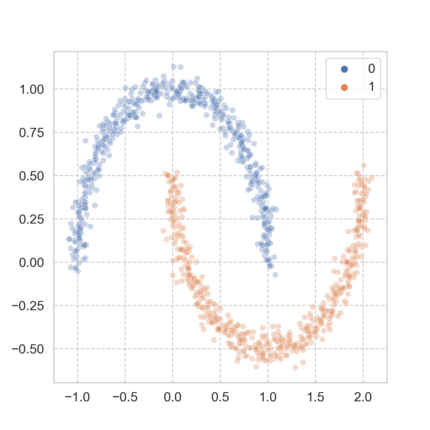
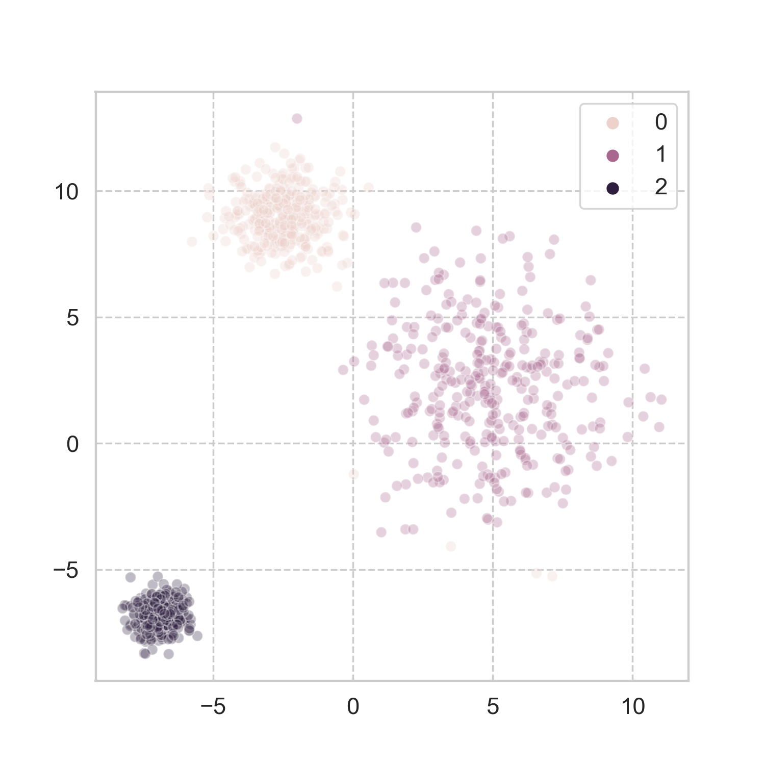
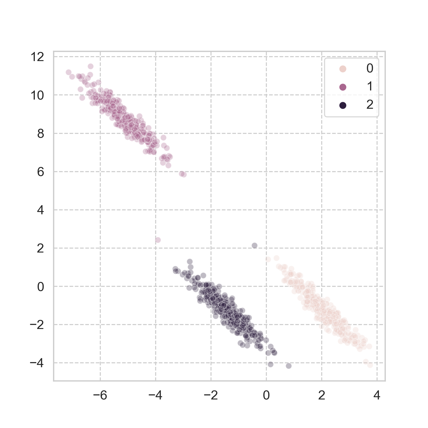
How does it work in more realistic problems? Taking a page from scikit-learn’s book, I used three of the datasets, and applied the aforementioned steps for spectral clustering (codes here). The results look pretty good to me.

Analogy in the physical world

It is hard for me not to put Time to the spectrum of a graph, and it turns out one could do that with our favorite simple harmonic oscillators. Imagine each vertex in the graph as a particle, and the edge connecting two vertices as a spring, whose spring constant equals the edge weight. Each particle’s mass equals the total degree of the vertex, and they are only allowed to move along the direction perpendicular to the plane of the graph. The subject of interest here is the motion of each particle, \(x_i\).

Here we are considering the ideal case, i.e., no energy loss due to friction. If one gives a little nudge to any of the particles, since all the particles are connected through various springs, the whole system will start to vibrate, and finally reaches some steady state that each particle is oscillating with a certain rhythm. I have discussed a similar case before, but here we are more interested in the case with more than just two masses. The question we want to answer is that: are there groups of particles that move in similar patterns? For example, imagine two groups of particles: the springs connecting the intra-group particles are very stiff, whereas the springs connecting the inter-group particles are very loose, then one would expect that the two groups will just oscillate independently with their own resonant frequency, regardless of the motions from the other group. Therefore it is very natural how the clusters should be decided.

Effectively, one wants to solve the below equation of motion (simple Newton’s second law and Hooke’s law):

\[L \textbf{x}(t) = - D \ddot{\textbf{x}}(t).\]

If one assumes a steady-state solution in the form of \(\textbf{x}(t) = u_k \cos(\omega_k + \theta_k)\), the system becomes:

\[D^{-1} L \textbf{u} = \omega_k^2 \textbf{u}.\]

This is exactly the problem that the normalized minimum cut aims to solve. The eigenvalues of the normalized Laplacian correspond to the resonant frequencies of the many-body system. The lowest eigenvalue of such system is always zero (corresponding eigenvector of \(\textbf{1}\)), that implies a static offset of all the particles. The second lowest eigenvalue and the corresponding eigenvector (also known as Fiedler vector) will tell us a great deal of the strongest collective motions of the system. Therefore one can run simpler clustering algorithm on the Fiedler vector in order to solve the original clustering problem.

References

There are only too many good resources on this subject. During the write-up of this post, I found this tutorial by von Luxburg very idiot-friendly (to me) yet comprehensive. Of course, the two seminal papers by Shi, Malik and Ng, Jordan, Weiss are very helpful too. The book by Fan Chung also occupied much of my free time.