Multi-armed bandit

You can play the 10-armed bandit with greedy, \(\epsilon\)-greedy, and UCB polices here. For details, read on.

Like many people, when I first learned the concept of machine learning, the first split made is to categorize the problems to supervised and unsupervised, a soundly complete grouping. Since then, I have mostly been dealt with the supervised problems, until the reinforcement learning becomes the hottest kid around the block.

Exploration vs exploitation trade-off

For a typical supervised learning problem, one usually trains models on a set of existing dataset (with labels), and then deploys the model to make predictions as new data are flowing in. In essence, the model only “learns” during the training stage, and leverage its knowledge ever since. Unless a new training session is triggered (for example with new training data), we simply keep exploiting.

Clearly this is not the ideal, at least not how human “learns”. We are constantly updating (training) our knowledge (model), often time through making mistakes when applying existing knowledge to a new situation, just like a new-born baby learning to walk. When asked to make a prediction (or decision), there are usually a handful of options one can choose from (is it a cat or dog, to go left or go right), and one will have to rely on a systematic framework to make the decision. But every decision will have some consequence (rewards), and we inevitably will reflect whether other decisions could have led to better outcomes. If so, when facing a similar situation again, we will make a better decision as we have learned from past experience. The hope is that, after enough such trial-ane-error, i.e, exploration, we would learn enough about the environment, and then commit ourselves to the best action going forward, i.e, exploitation.

This learning framework, namely, reinforcement learning, sounds similar to supervised learning, but differs in a subtle yet fundamental manner. Here, when one is “exploring”, she is not only collecting the data (with the rewards as labels), but also immediately apply this latest learning when making the next prediction/decision. In a sense, the online method in supervised learning carries the same virtue, as it also updates the underlying model’s parameters as new data streaming in, but the reinforcement learning framework has this characteristic baked-in natively.

The multi-armed bandit problem

The classic example in reinforcement learning is the multi-armed bandit problem. Although the casino analogy is more well-known, a slightly more mathematical description of the problem could be:

As an agent, at any time instance, you are asked to make one action out from a total of \(k\) options. Taking each of the options will return some numerical reward, according to their respective underlying distributions. The question is, what is the policy the agent should apply, such that it will maximize the total reward in the long run?

The environment (arms)

It helps to make the problem, especially the “arms”, concrete. Below we made a 10-armed environment. Each arm’s return follows a Gaussian distribution with variance of 1. The mean of each arm, \(\mu_i\) where \(i\) = 0..9, is drawn from a standard Normal distribution. Below is an example of such an environment.

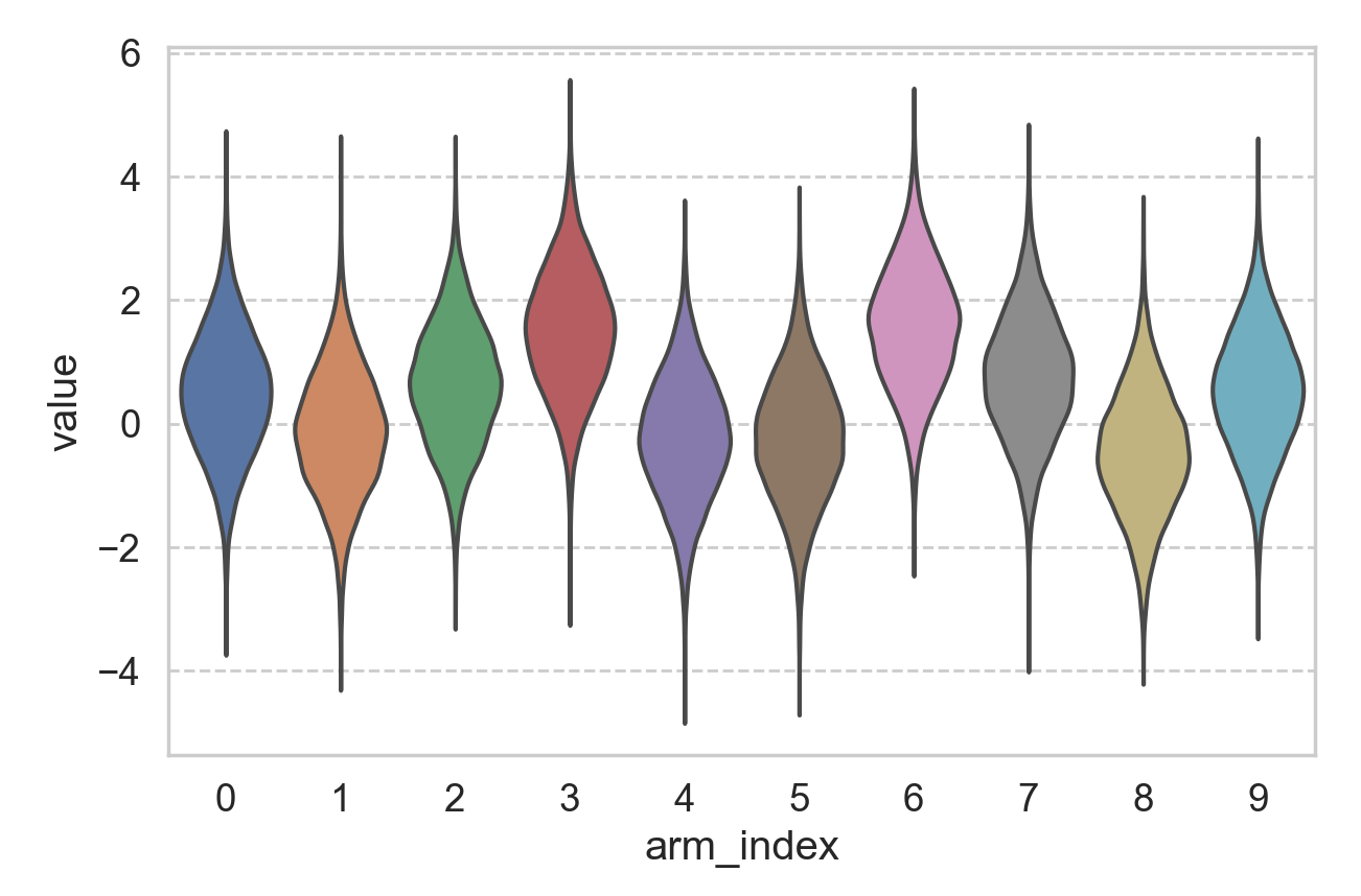
As an agent, my goal is to achieve the largest long-term reward, and if I know all the 10 distributions, I would pull arm #6 all the time, as it has the largest mean (about 1.58). However, I would not know the underlying distribution, as the question is what policy should I apply, if I have infinite number of attempts, in order to end up pulling arm #6 in the long run?

Since I can pull infinite number of times, how about I pull each arm, say, 100 times, and starting from the 1001\(^{\text{th}}\) attempt, I will pull the arm that has given me the highest average reward (from the 100 trials). By the law of large numbers, I will most likely end up pulling arm #6 in the end, but the previous 1000 pulls (or 900 if discount the times we pull on arm #6) seem quite wasteful. Under such a policy, we probably explore too much.

Greedy and \(\epsilon\)-greedy policy

The pursuit to explore less sets up us nicely to the greedy policy. Namely, we will try to assign a value to each arm, say as \(Q_i\), and update our estimate of \(Q_i\) each time after we pull arm \(i\) and get a reward. When making the decision for which arm to pull next, we simply “greedily” pull the one that has the highest value, namely, \(\text{argmax}_i{Q_i}\).

A critical step here is to update \(Q_i\). The simplest implementation is to use the averaged past reward as \(Q_i\). Assume that there are only 2 arms, each has been pulled 3 times. Arm #1 gives reward as [3, 4, 3], and arm #2 as [2, 5, 4]. Then our estimate for \(Q_1\) will be 3.33, and for \(Q_2\) will be 3.67. Therefore, under the greedy policy, for the 7\(^{\text{th}}\) pull, we will go with arm #2. Say this time we are not so lucky as arm #2 returns 0, then we have to update our estimate of \(Q_2\) to 2.75, such that for the next pull, arm #1 becomes a better option, we just need to update \(Q_1\) after the pull. You get the idea.

But only committing to the arm with the highest value estimate, seems a little bit myopic, as we might be exploiting too much. A natural extension is to allow some exploration, such that when deciding which arm to pull next, with a small probability (\(\epsilon\)), we will not pull the one with the highest value estimate, but a random different arm. This modification constitutes the key idea of the \(\epsilon\)-greedy policy, in which we try to strike a balance between the exploration-exploitation trade-off. the value of \(\epsilon\) will be a hyper-parameter for the algorithm.

Comparison between different policies

Both policies make intuitive sense, but we still need a quantitative framework for comparisons. Enter the power of numerical simulation. Once we have created an artificial environment as a testbed, we can put an agent into such an environment and deploy the policy of interest. However the world is inherently stochastic, therefore even the best policy might yield a worse outcome, than a sub-optimal policy, for a given trial. Therefore, a more proper method to compare different policies, is to compare the average outcome with the same policy, from multiple simulations where each simulation is run with its own, independent environment.

Below we show such averaged results, from 2000 simulation for single policy (code, quick-start notebook). The environment used here is the 10 Gaussian arms mentioned above. The policies that are examined here are greedy, \(\epsilon\)-greedy, and upper confidence bound (UCB), which we will discuss shortly.

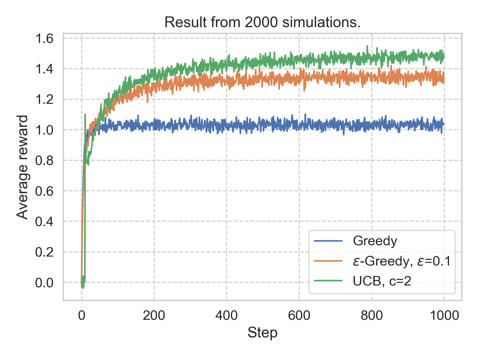
The first observation is that, under all the policies yield rewards larger than 1 in the long run. This is comforting as a non-policy (randomly choose an arm) should lead to an expected reward of 0. The second observation is that, in this case, a \(\epsilon\)-greedy policy with \(\epsilon\) = 0.1 seems to outperform the simple greedy policy.

Upper confidence bound (UCB) policy

What is the UCB policy that seems to beat both greedy and \(\epsilon\)-greedy algorithms? The idea is pretty intuitive: previously we use the averaged past reward as the point estimate the value, \(Q_i\), for each arm, and for next action, we pick the arms whose point estimate is the largest. In UCB we are instead choosing the arm whose value could be the largest. In essence, we assign a confidence interval to \(Q_i\), and pick the arm with the highest upper confidence bound of \(Q_i\). More precisely, the arm to pull, at time step \(t\), \(A(t)\) is:

\[A(t) = \text{argmax}_i[Q_i(t) + c\sqrt{\frac{\ln{t}}{N_i(t)}}],\]

where \(Q_i(t)\) is the point estimate of \(Q_i\) prior to step \(t\), and \(N_i(t)\) is the number that arm \(i\) has been pulled prior to step \(t\). \(c\) is a hyper-parameter to control the size of the confidence interval.

We see that, everything else being equal, if a less-pulled arm would have a higher upper confidence bound than other arms that have been pulled more often, and we would prefer this arm precisely because we are less certain about its payoff. But we believe it would give us higher reward. Again, as in most machine learning problem, the exact setting and hyper-parameter tuning would matter quite a lot.

Conclusion

The multi-armed bandit is such a classic problem yet I always find it a bit elusive – the casino analogy fuels its popularity. Not until I implemented the codes and ran the simulations to see the results myself, that it becomes clear. Also this post is inspired by the book Reinforcement Learning: An Introduction, by Richard S. Sutton and Andrew G. Barto. This blog post also offers an excellent explanation, using a slightly different example.