The model to flatten the curve

You can make you own curve here. We have also made a website to track the daily \(R_0\) for all counties in US here. For details, read on.

As the current covid-19 pandemic sweeping across the global (certainly in New York) and posting dreadful tallies day over day, most of the governments are urging their citizens to stay home, practice the social distancing, in order to “flatten the curve”, so that we can get out from this crisis.

Why we need to flatten the curve

The curve referenced here usually refers to the number of hospitalizations over time. Being a respiratory disease, the covid-19 patients often require care with medical resources, such as hospital staff and ventilators. The problem is, once the number of patients overwhelms the medical resources in the area, there is almost nothing the doctors can do, but forced to make difficult and agonizing decisions [1].

In order to avoid such meltdown of medical system, the key is to slow the transmission of the disease among the population, such that the rush to the hospitals is spread out over time. Qualitatively, this makes perfect sense, however, how does one calculate the curve quantitatively, namely, put the numbers on the axes?

The model that draws the curve

The most commonly used framework in modelling infectious disease is the SIR model. The basic construct of the model is pretty simple: the whole population is divided into different “compartments”, and any person at any given time is in one of those buckets. In the most basic setting, there will be three compartments: Susceptible (not yet have the disease), Infectious (have the disease), and Recovered (immuned). A person will move from one compartment to another as time progresses, and the dynamic (rate) of people moving between different compartments dictates the total number of people in each compartment. This dynamics will help us to draw the curve.

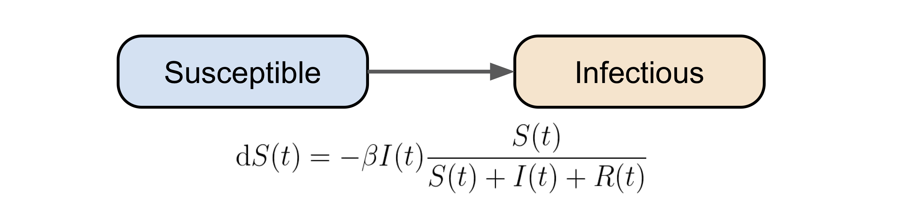
From S to I

At a given time \(t\), if the total number of infectious people is \(I\), then the number of people they can infect (hence being turned to infectious) can be described as \(I(t) \beta \frac{S(t)}{S(t) + I(t) + R(t)}\). The term \(\beta\) is the probability of transmission from an infectious person to a susceptible person, and the last term is the proportion of the susceptible people in the whole population. In this dynamical system setting, \(\beta\) can be considered as the “infection rate”.

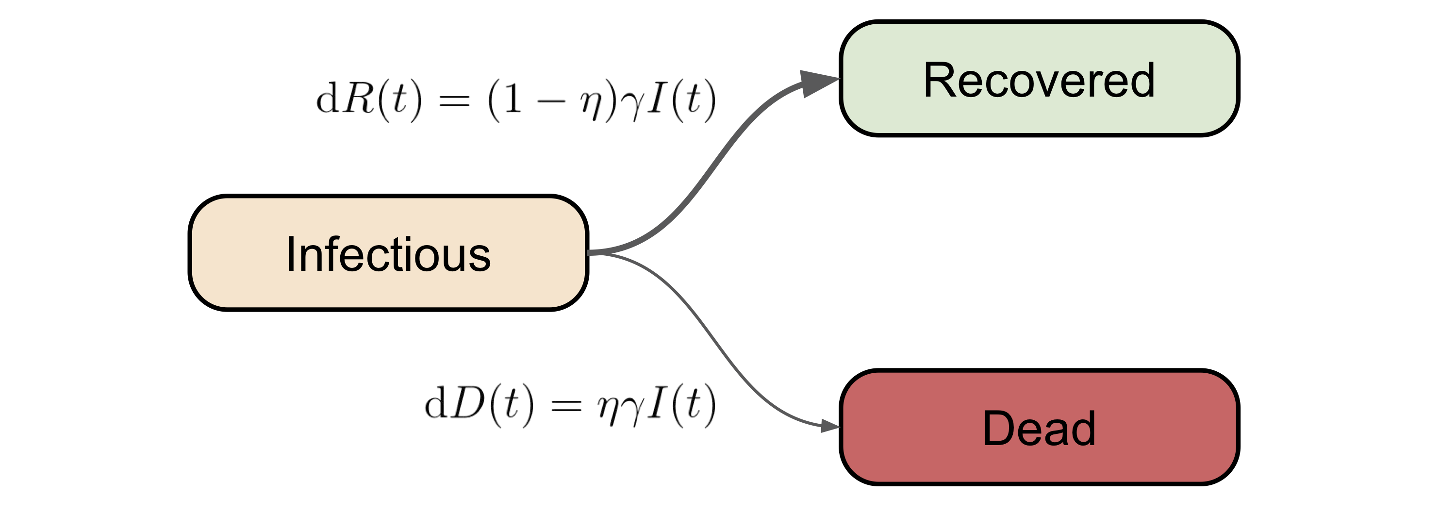
From I to R (or D)

Once a person becomes infectious (not necessarily symptomatic), the next compartment(s) for him/her to go is recovered, or unfortunately, dead. Note that in the vanilla version of the SIR model, death is not considered, however, given the unusally high fatality rate of covid-19 [2], we can not ignore the non-zero death rate.

With the above consideration in mind, we will assume the number of people moving from \(I\) to \(R\) is \((1-\eta) \gamma I(t)\), and the number of people moving from \(I\) to \(D\) is \(\eta I(t)\). Again, in this dynamical system setting, \(\gamma\) and \(\eta\) can be treated as the (quasi-)recovery rate and death rate (due to the disease), respectively.

Putting everything together

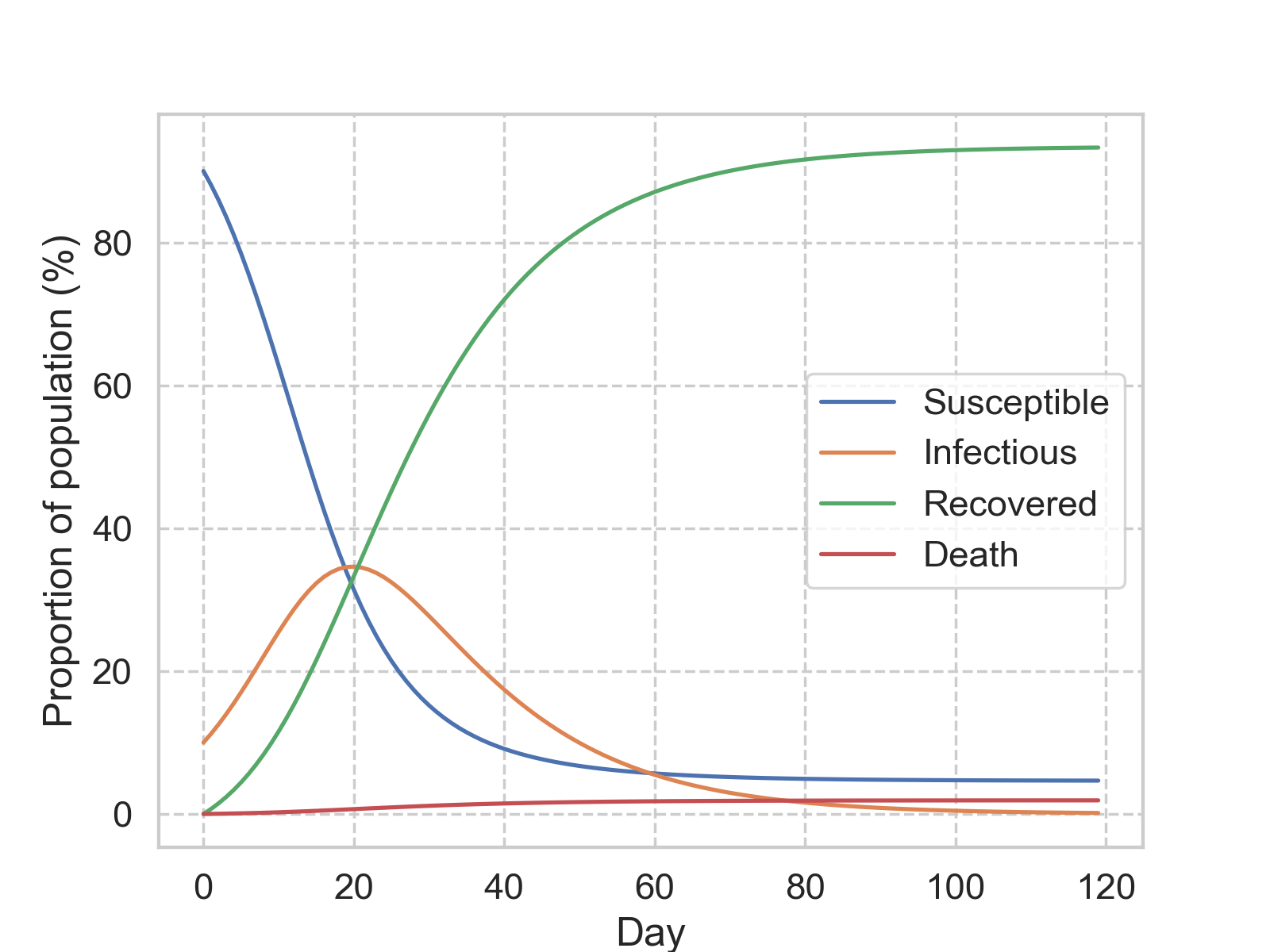
Now we have all the ingredients of this SIR(D) model in place, the next thing is to properly describe their dynamics between each other (\(S, I, R, D\)), shown as the odinary differential equation (ODE) below:

\[\begin{split} \text{d}S(t) &= -\beta I(t) \frac{S(t)}{S(t) + I(t) + R(t)}\\ \text{d}I(t) &= -\text{d}S(t) - \gamma I(t)\\ \text{d}R(t) &= (1-\eta) \gamma I(t)\\ \text{d}D(t) &= \eta \gamma I(t) \end{split}.\]

This can be easily solved numerically (python code). Below is a simulation with \(\beta\) = 0.21, \(\gamma\) = 0.07, and \(\eta\) = 0.02.

The most commonly used time step is a day, and with this setting, we can layer in some statistical assumption to bring more meanings to the parameters. Suppose the duration of each infection is exponentially distributed, with an average of \(c\) days. Then on average, we would expect \(I/c\) people recovered every day. Therefore, the recovery rate, \(\gamma\) can be approximated with \(1/c\).

The famous R0

Another number that is being discussed a lot in the pandemic context, is the basic reproduction number, \(R_0\). Simply put, \(R_0\) is the averged number of susceptible people that an infectious person can transmit the disease to. Conceptually, \(R_0\) describes the rate of \(I\), as we can see by re-arrange \(\text{d}I\) as:

\[\begin{split} \text{d}I(t) &= \beta I(t) \frac{S(t)}{S(t) + I(t) + R(t)} - \gamma I(t)\\ &= (\frac{\beta}{\gamma}\frac{S(t)}{S(t) + I(t) + R(t)} - 1) \gamma I(t) \end{split},\]

where we can define \(R_0 = \beta / \gamma\). By doing so, and further assuming \(I \approx R \approx 0\) at the beginning of the outbreak, the above equation can be reduced to:

\[\text{d}I(t) = (R_0 - 1)\gamma I(t).\]

This simplified form distills the essence of the meaning of \(R_0\): if it is larger than one, then one should expect to see more and more infected people, whereas one should aim to bring \(R_0\) below one, to bring the number of infectious people (hence dead) down over time. This alone can explain the importance of social distancing!.

There is an important note we should take about \(R_0\), that \(R_0\) is not easy to measure as the reality is much more complicated than this simple model and the assumptions we impose. From our simplification here, we can see that it is the ratio between the infection rate and the recovery rate, and given that we can treat \(1/\gamma\) as the average number of days of recovery, which can be approximated with the number of hospitalized days, one can use collected data, and an assumed \(R_0\), to solve the ODE completely.

Parameter estimation and model extension

While the construct and the (numerical) solution of the model is relatively straightforward, the real complexity lies in the parameters estimation, e.g., what is the most appropriate values to use for \(\beta, \gamma, \eta\). One can infer their values by fitting data observed so far. Also bear in mind that these parameters can be time-dependent, as the dynamic of the pandemic, or social policies change.

Aside from the intricacy in parameter estimation, another note worth mentioning here is that, one can extend the current SIR(D) model with more compartments, such as hospitalized, intensive-care-unit’ed (ICU’ed), as long as one can properly model the transition between each compartment, and estimate the parameters with reasonably good accuracy.