Statistical tests for multiple comparisons

Can you also run the comparison along this dimension?

I believe this is a common question that is asked to a data scientist or data analyst. Say your company has just run an A/B test, aiming to find whether a blue button leads to more conversions than a red button. Millions of clicks later, there seems to be no significant difference. Disappointed, the program manager believes we can still draw some meaningful conclusions: maybe the blue button indeed leads to more conversions among female users, or among users from New York, or among … This strip from xkcd perfectly captures this spirit.

What is wrong with that

Of course, there is no magic about the green beans. The culprit here is the type I error, whose probability is quantified by the p value. The common practice is to reject the null hypothesis (hence accept the alternative hypothesis) only if the p value is less than a pre-determined threshold (usually 0.05). However, such routine becomes problematic when we perform multiple tests on the same dataset.

To drive this point home, let’s do a simple simulation.

We first prepare a random vector \(Y\) that is drawn from a uniform distribution \(\it{U}(0, 1)\), so that we know the null hypothesis is true.

import numpy as np
np.random.seed(10)

n_samples = 10000
Y = np.random.random(n_samples)

Next, let’s add some “colors”, namely, create a set of random 0/1 covariates, to “describe” the vector \(Y\).

import pandas as pd

n_trials = 500
X = []
for _ in range(n_trials):
    X.append(np.random.randint(2, size=n_samples))

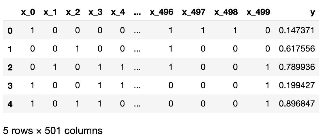
data = pd.DataFrame(np.array(X).T)
data.rename(columns={c: f'x_{c}' for c in data.columns}, inplace=True)
data['y'] = Y

With the help of pandas, we can put the dataset nicely together, with the first 5 rows shown below. In total, we have 10000 rows of observations (\(y\)).

Since we know exactly how \(y\) is generated, no matter which dimension is chosen, we know the null hypothesis is always true. However, if we run all 500 comparisons, by virtue of the definition of p value, we are bound to draw some statistically significant conclusions, if we only rely on obtaining small p values.

from tqdm import tqdm
from typing import List
from scipy import stats

def multiple_comparisons(
		data: pd.DataFrame,
		label: str = 'y') -> List[float]:
    """Run multiple t tests."""
    p_values = []
    for c in tqdm(data.columns):
        if c.startswith('y'):
            continue
        group_a = data[data[c] == 0][label]
        group_b = data[data[c] == 1][label]

        _, p = stats.ttest_ind(group_a, group_b, equal_var=True)
        p_values.append((c, p))

    return p_values

p_values = multiple_comparisons(data)

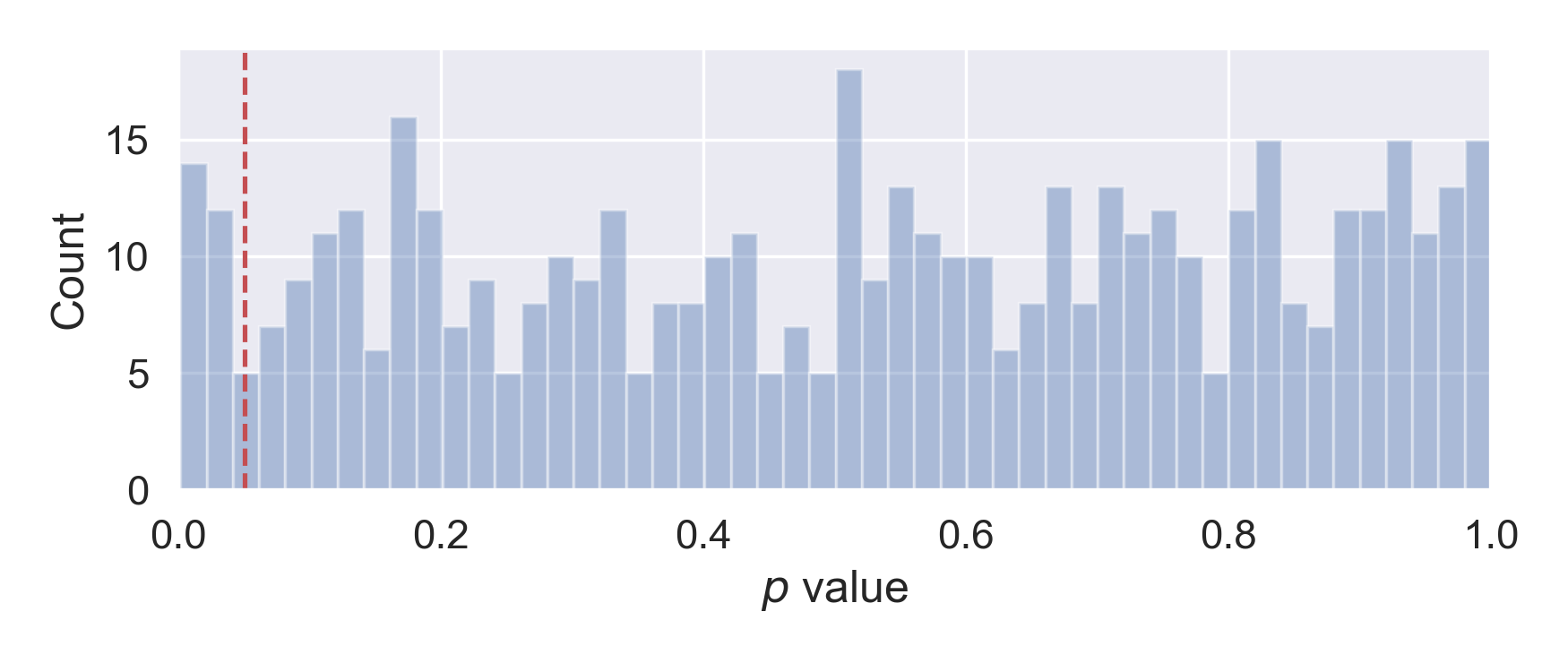
If we examine the distribution of the 500 p values, we will find it to be more or less uniform across [0, 1], as expected. Therefore, if we choose 0.05 as the type I error rate \(\alpha\), we will make about 25 false discoveries.

A simple fix: Bonferroni correction

It seems that, when we are conducting a family of tests on the same dataset, the chance of getting false positives becomes larger. In fact, if there are \(m\) comparisons carried out, then the probability of getting no type I error from all the comparisons is simply \((1 - \alpha)^m\). Thus the probability of getting at least one type I error is \(1 - (1 - \alpha)^m\). Even for a medium value of \(m\), this probability (family-wise error rate) can be surprisingly large.

To control for that, one needs to be more strict when deeming “statistically significant”. The Bonferroni correction is arguably the simplest fix: for each of the \(m\) comparisons, adjust \(\alpha\) to \(\alpha / m\). Then, only when an observed p value that is smaller than \(\alpha / m\), we reject the null hypothesis.

If we use the Bonferroni correction to our running example, namely, using 0.0001 as the critical value, we will reject 0 test, as we should.

# bonferroni correction
print('Total number of discoveries is: {:,}'
      .format(sum([x[1] < threshold / n_trials for x in p_values])))
print('Percentage of significant results: {:5.2%}'
      .format(sum([x[1] < threshold / n_trials for x in p_values]) / n_trials))

# Total number of discoveries is: 0
# Percentage of significant results: 0.00%

Get the power back: Benjamini–Hochberg procedure

The major disadvantage of the Bonferroni correction is that, it is too conservative. It trades the power for the low family-wise error rate. To illustrate this drawback, let’s make half of the 500 comparisons with true differences.

To do so, we take the first 250 features, for each of them, whenever there is an 1, we draw a sample from an \(N(1, 1)\), and add it to y. If there is a 0, we do nothing. Essentially, we create 250 independent \(N(1, 1)\), each of 10000-long, and then multiply this (10000, 250) matrix, element-wise, to the first 250 columns of the dataset. By doing so, when we conduct a comparison along any of the first 250 dimensions, we should get a significant result.

n_true_features = n_trials // 2

offset = np.random.normal(loc=1., size=(n_samples, n_true_features))
offset_sum = np.multiply(
    offset,
    data[data.columns[:n_true_features]].values).sum(axis=1)
Y2 = Y + offset_sum

data['y2'] = Y2

p_values = multiple_comparisons(data, label='y2')

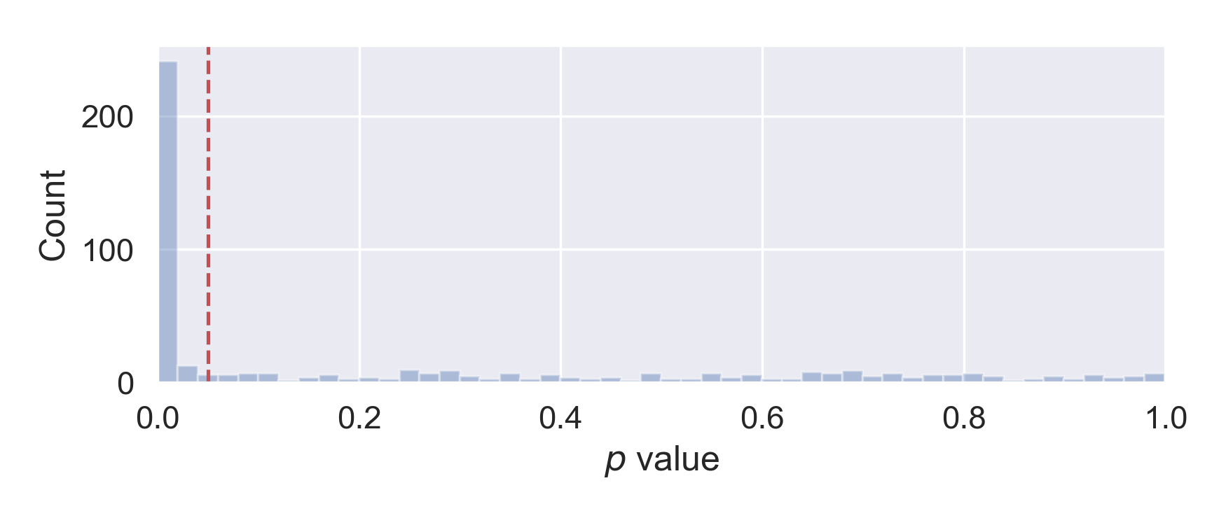
Let’s make the histogram of the corresponding p values, as shown below. We can indeed find about half (259) of comparisons with p value less than 0.05. This is exactly what is expected, as 250 + false positives (=13 ~ 250 * 0.05) - false negatives (~11, see last section for estimation).

However, if we apply the Bonferroni correction, which uses 0.0001 as the critical value, we will only get 99 significant results. They are all from the first 250 dimensions, so we are not making any false discoveries, at the expense of 151 false negatives. It clearly shows that we have less (statistical) power.

To get the power back, one can apply the Benjamini–Hochberg procedure. The process is quite simple too: once we get all the p values from the \(m\) comparisons, first rank them from low to high. Then traverse from the smallest p value, and see whether it is smaller than \(\frac{i}{m} \alpha\). Until this condition is not met, all the preceding comparisons are deemed significant.

# Benjamini–Hochberg procedure
p_values.sort(key=lambda x: x[1])

for i, x in enumerate(p_values):
    if x[1] >= (i + 1) / len(p_values) * threshold:
        break
significant = p_values[:i]

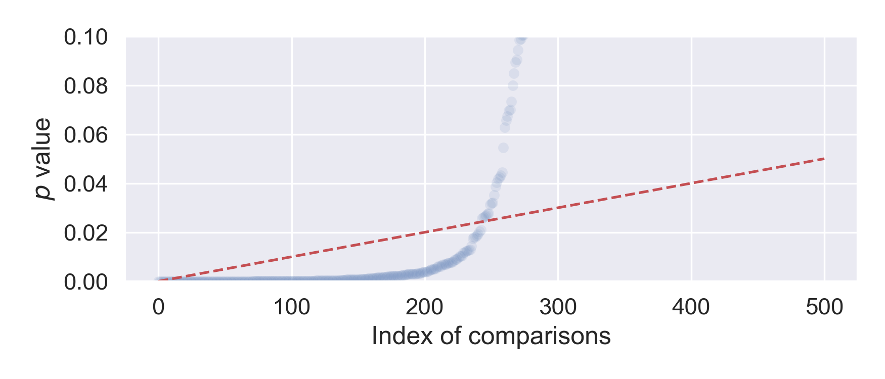
Pictorially, we plot the sorted p values, as well as a straight line connecting (0, 0) and (\(m\), \(\alpha\)), then all the comparisons below the line are judged as discoveries.

The figure below shows the result from our running example, and we find 235 significant results, much better than 99 when using the Bonferroni correction. Among the 235 discoveries, there are 9 false positives, hence we are also getting 24 false negatives.

By using the less stringent, yet simple Benjamini–Hochberg procedure, we recover the statistical power lost from the Bonferroni correction. However, one still needs to check for the assumptions, and exact use cases.

Estimation of False Negatives

I think this is a bit of brain gymnastics. Recall that we create the Y2 vector as the sum of a uniform \(\it{U}(0, 1)\), and 250 modified Normal distribution, with mean of 1 and variance of 1, such that \(Y_2 \sim \it{U}(0, 1) + \sum_{k=1}^{250}Z_k\). When the alternative hypothesis is true, the expected difference will be 1, but we also want to know its variance.

Here we will mainly use the formula for the variance, as:

\[\mathrm{Var}[X] = \mathrm{E}[X^2] - \mathrm{E}[X]^2.\]

Here each of the \(Z_k\) is independent of each other, so we can conveniently calculate the variance of \(\sum_{k=1}^{250}Z_k\) from \(Z_k\). Recall that \(Z_k\) is created as the product of a Bernoulli trial with \(p = \frac{1}{2}\), and a draw from \(\it{N}(1, 1)\). Therefore we have \(\mathrm{E}[Z_k] = \frac{1}{2}\), and \(\mathrm{Var}[Z_k] = \mathrm{E}[Z_k^2] - \mathrm{E}[Z_k]^2\). In the variance equation, the former can be calculated from the expectation, where we use the fact that \(\mathrm{E}[X^2] = 2\) for \(X \sim \it{N}(1, 1)\). This leads to \(\mathrm{Var}[Z_k] = \frac{3}{4}\).

Finally, we arrive at \(\mathrm{E}[Y_2] = 125.5\), and \(\mathrm{Var}[Y_2] = \frac{1}{12} + 250 \times \frac{3}{4}\). We will use this variance to approximate the variances of both the test groups. From here, it is just a short derivation to the number of False Negatives, using the number of total samples (10000) and the total number of comparisons (250).

All the above calculations can be found in this notebook.