
The secretary problem
I was reading the book Algorithms to Live By for the second time recently, and finally decided to take a deeper look at some the questions posted inside. There is no more enticing problem than the first example brought forward by the authors, the secretary problem.
The problem
The setting is rather straightforward: you need to hire a secretary (or an analyst, a data scientist), and you only have the time/financial budget to interview at most \(N\) candidates.
Here come the crucial twists. First, you can only rank all the interviewed candidates ordinally, without any knowledge of their standings in the hidden, total candidate pool. In other words, the best candidate you have seen so far may or may not be the best candidate you can ever interview. Second, after interviewing each candidate, you have to make the hire/no-hire decision right away. If you decide to hire, the whole process is finished, and if you decide to pass on this candidate, you can not go back to him or her again.
The second constraint turns the decision making the process more like a bet. For example, although the one you just interviewed is the best so far, he or she is just the third of 20 candidates you are interviewing, shall you make the hiring call? Is there a non-random strategy one can follow here?
Look-then-leap
There are many sensible strategies one can propose here, for example, after you have seen but let go of a good candidate, if you have seen more than \(x\) consecutive candidates than the previous “benchmark”, hire the next who is better than the benchmark. However, the simplest strategy here, is the so-called look-then-leap: you just interview the first \(r\) candidates, without hiring anyone from them. Then starting from the \((r+1)^\text{th}\) candidate, hire the first one who is better than the best of the first \(r\) candidates. In essence, the first \(r\) candidates establish a reference for you to make the final decisions. Of course, if the best among the first \(r\) candidate happens to be the best among all, then you are luck out, and have to hire the last candidate you interview, assuming you have to hire someone.
Since we are dealing with a stochastic process here, the objective here would be to maximize the probability of hiring the best candidate. Even we have devised the structure of the strategy, there is still the question of what value of \(r\) to use. To be more general, the value we are interested in is the ratio, \(r/N\), namely, the proportion of candidates to interview before any hiring decisions. It turns out the optimal value is the magical \(1/e\).
Seeing is believing
Given the seeming simplicity of this strategy, it is hard to resist the temptation of running the “brute-force” simulations, just to see the probabilities of hiring the best candidates, when using different proportions. It is fairly straightforward to code up, as shown here.
In the simulation settings, we set \(N\) = 1000 (number of total candidates), and let the threshold (\(\left \lfloor{r / N}\right \rfloor \)) changes from 0.01 to 0.99 with 0.01 step size. For each threshold, we will permutate the sequence of the incoming candidates for 10,000 times while applying the same strategy. Only if the best candidate is hired, then we will call the trial a success.
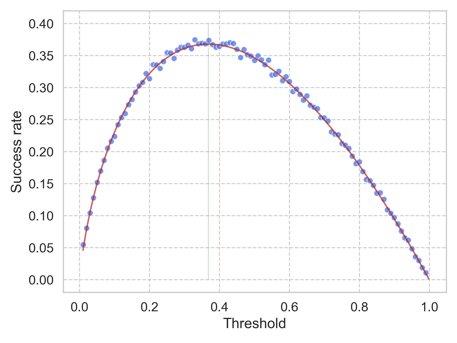
The simulated success rate for each threshold is shown in the figure above. The details can be found in this notebook. The red vertical line corresponds to the value of \(1/e\), and the red solid curve shows the result of Equation \(\eqref{eq_integral}\) (see next section). It fits rather well with the aforementioned theory, that \(1/e\) is the best threshold to use for this look-then-leap policy.
View from the probability lens
It is intelligently irresponsible not to ask why \(1/e\) is the magical answer. It turns out one only has to resort to conditional probability to arrive at the answer.
Under the look-then-leap policy, the objective function one tries to maximize is the probability of selecting the best candidate \(P(r; N)\), where \(r\) is the “number of looks”, and \(N\) is the total number of candidates. Then in mathematical language, we have:
\[\begin{align*} P(r; N) &= \sum_{i=1}^N P(i\text{ is selected}, i \text{ is the best}) \\ &= \sum_{i=1}^N P(i\text{ is selected}~|~i\text{ is the best}) ~\times P (i\text{ is the best}). \end{align*}\]We simply assume the last term as \(1/N\), as the best candidate can be at any location in the \(N\) sequence, with equal probability. After moving this part out from the summation, we can further expand the remaining part using our policy, as:
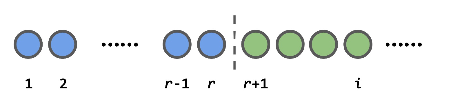
\[\begin{align*} ~&\sum_{i=1}^N P(i\text{ is selected}~|~i\text{ is the best})\\ =& \sum_{i=1}^r 0 + \sum_{i=r+1}^N P(i\text{ is selected}~|~i\text{ is the best})\\ =& \sum_{i=r+1}^N \frac{r}{i-1}. \end{align*}\]The zero probability for the first \(r\) items is quite straightforward: if the best candidate happens to be in the first \(r\) (i.e, \(i \le r\)), then we are luck out. The interesting part is from the second summation: if the best candidate is not in the first \(i\), then under our policy, the only condition that it will be picked is that, the second best candidate in the first \(i-1\) is in the first \(r\), and the probability for this condition is \(r/(i-1)\). Note that here we only require the second best candidate in the first \(i-1\), instead of that of the \(N\) since we are dealing with conditional probability here. The illustration below should help to demonstrate this logic.
Coming back to \(P(r; N)\), now we have:
\[\begin{equation} P(r; N) = \frac{r}{N} \sum_{i=r+1}^N \frac{1}{i-1} \tag{1}\label{eq_master}, \end{equation}\]and the goal will be for a given \(N\) to find the \(r\) that maximize \(P(r; N)\). However, for the sake of analytical purposes, we want to explore the limit where \(N \rightarrow \infty\), what’s the optimal threshold \(t = r/N\). By doing so, the summation is converted to the integral as:
\[\begin{align*} P(r; N) &= p(t) \\ &= t\int_x^1 \frac{1}{x} \text{d}x \\ &= -t \ln(t), \tag{2}\label{eq_integral} \end{align*}\]whose maximum can be easily found at \(t = 1/e\), with \(p(1/e) = 1/e\). Not surprisingly, the plot of \(-t \ln(t)\) agrees nicely with the numerical simulations.
View from the dynamic programming lens
All the preceding derivations are all nice, except for that we already assume the “look-then-leap” strategy is optimal, whereas one only has to hone in the details. But can one prove the assumption?
Of course one can, just some brain gymnastics exercises. The key here is to properly describe the state and value of the process. For this case, we need two numbers to express a state: \(r\) and \(s\), where \(r\) is the number of candidates we have seen so far, and \(s\) is the apparent ranking of the last, i.e., the \(r^\text{th}\) candidate. The value function, \(V(r, s)\) that is being sought here, is the maximum expected probability of choosing the absolute best candidate when the state is (\(r, s\)). As usual, there are \(N\) total candidates to be considered.
After having all the semantics in place, the crucial next step is to derive the logical relation of the value function between different states. Since there are only two state variables, it allows us to visualize the whole dynamic programming logic in a matrix form, as seen below.
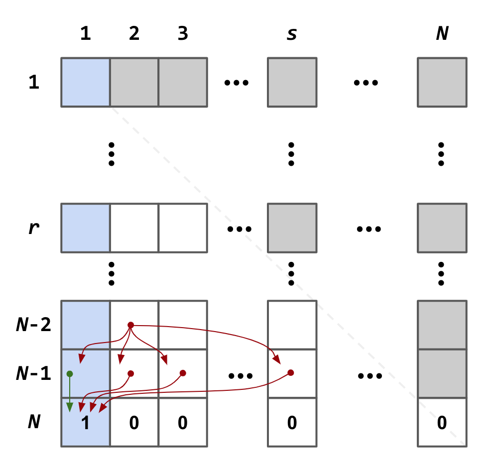
The row and column indices of the matrix indicate \(r, s\), respectively, whereas the value of each element of the matrix is the value function \(V(r, s)\) as defined above. Due the nature of this problem, almost half the elements (namely, the upper right half) have no real meanings.
What if we have interviewed all candidates
As in a typical dynamic programming scenario, we will start from the edge, as in this case, the last row. Here, the last row holds the maximum expected probability of selecting the best candidate, when in the state (\(N, s\)). Apparently, we can only “win” when \(s = 1\), with probability of 1. Therefore, we can populate the last row with only the first element set to 1, as \(V(N, 1) = 1\), and zeros for the rest.
What if we have interviewed all but one candidates
Now let’s move back the penultimate row, in which case we have observed all but one candidate. If the \((N-1)^\text{th}\) candidate’s apparent ranking is not 1, we have no other choice but keeping interviewing the last candidate, hoping to arrive at the magical (\(N, 1\)) state. Since there is a probability of \(1/N\) that the last candidate is the best, then the probability of winning at the state (\(N-1, s\)) where \(s \neq 1\) is then:
\[\begin{align*} V(N-1, s) = \frac{1}{N}V(N, 1), ~~~\text{for}~s = 2, 3, ..., N-1.\tag{3.1}\label{eq_dp_penultimate_1} \end{align*}\]If we are in the state of (\(N-1, 1\)), there is an interesting decision have to be made: shall one end the search and pick this candidate, or keep searching? Given that we have observed \(N-1\) candidates and this last one has the apparent ranking of 1, it is very likely that his or her abosulate ranking is also 1. Actually, the probability of this \((N-1)/N\), that is, if we stop here, the winning probablity is \((N-1)/N\). Of course, one can keep searching, hoping the last candidate can be even better, i.e., to end up in the (\(N, 1\)) state. As described above, the probablity of such occurence is \(1/N\). Putting these two cases together, we have for (\(N-1, 1\)):
\[\begin{align*} V(N-1, 1) = \max{[ \frac{N-1}{N}, \frac{1}{N}V(N, 1) ]}.\tag{3.2}\label{eq_dp_penultimate_2} \end{align*}\]Generalization and the Bellman equations
From the two simple exercises above, it is clear that one needs to distingusih the state (\(r, 1\)), and state (\(r, s\)) where \(s \neq 1\). For the latter, one has no choice but to keep going. Since the apparently ranking of the \((r+1)^\text{th}\) can be anywhwere between 1 and \(r+1\) with equal probability, as one is eqaully likely to capature the value of \(V(r+1, s')\) where \(s' = 1, 2, ..., r+1\). Therefore, the value function at state (\(r, s\)) for \(s \neq 1\) is:
\[\begin{align*} V(r, s) = \sum_{s'=1}^{r+1} \frac{1}{r+1} V(r+1, s'), ~~~\text{for}~s = 2, 3, ..., N-1, \tag{4.1}\label{eq_dp_bellman_1}. \end{align*}\]Note that, Eq. \eqref{eq_dp_bellman_1} is the generalized case for \(r = N-1\), namely, Eq. \eqref{eq_dp_penultimate_1}.
As for the state (\(r, 1\)), one always has the option of stopping and reaping the winning probability of \(r/N\), or keep going, which folds into the situation that we just discussed in Eq. \eqref{eq_dp_bellman_1}. Therefore, the value function at state (\(r, 1\)) is:
\[\begin{align*} V(r, 1) = \max{[ \frac{r}{N}, \sum_{s'=1}^{r+1} \frac{1}{r+1} V(r+1, s') ]}. \tag{4.2}\label{eq_dp_bellman_2} \end{align*}\]We have done the hard logical derivations, and what is left are just some simple arithmetic. It is not hard to extrapolate, for \(r < N\):
\[\begin{align*} V(r, s) &= \frac{r}{N}(\frac{1}{r} + \frac{1}{r+1} + ... + \frac{1}{N-1})\\ &= \frac{r}{N}\sum_{i=r}^{N-1} \frac{1}{i}, ~~~\text{for}~s \neq 1, \tag{5.1}\label{eq_dp_bellman_final_1}\\ V(r, 1) &= \frac{r}{N}\max{[1, \frac{1}{r} + \frac{1}{r+1} + ... + \frac{1}{N-1}]}\\ &= \frac{r}{N}\max{[1, \sum_{i=r}^{N-1} \frac{1}{i}]}. \tag{5.2}\label{eq_dp_bellman_final_2} \end{align*}\]Optimal strategy
As we have interviewed \(r\) candidates, we are equally likely to be at any of the (\(r, s\)) states, each with probability of \(1/r\). Since we will only stop if we hit the (\(r, 1\)) state, and there is a \(\max\) function in \(V(r, 1)\), we are more interested how this \(\max\) is triggered with different \(r\). Note that, the function \(f(r) = \sum_{i=r}^{N-1} \frac{1}{i}\), it is monotonic decreasing, therefore, once its value dips below 1 (as we are interviewing more candidates), the best bet is stop searching as soon as we are in the (\(r, 1\)) state, as the \(1\) term in the \(\max\) function will take dominance. Essentially, one is looking for an \(r_o\), such that \(f(r_o) > 1 \geq f(r_o + 1)\).
This, finally, justifies the “look-then-leap” strategy: we will keep looking (increasing \(r\)), until we pass the critical value of \(r_o\), then we are ready to commit ourselves, for the next candidate with the apparent ranking of 1. Since for the first observation after \(r_o\), the probability of arriving at state (\(r_o + 1, 1\)) is simply \(1/(r_o + 1)\), and when we do, the winning probability is \((r_o + 1)/N\); when one arrives any of the other (\(r_o + 1, s\)) states, we will have to proceed to (\(r_o + 2, s\)) states, from which we have \(1/(r_o + 2)\) chance of reaching the (\(r_o + 2, 1\)) state and stop, or \((r_o + 1)/(r_o + 2)\) chance to keep going. Taking the expected value of this recursive series, we have:
\[\begin{align*} P(r_o; N) &= \frac{1}{r_o + 1} \frac{r_o + 1}{N} + \frac{r_o}{r_o + 1}P(r_o + 1; N)\\ &= \frac{1}{N} + \frac{r_o}{r_o + 1}(\frac{1}{r_o + 2}\frac{r_o + 2}{N} + \frac{r_o + 1}{r_o + 2}P(r_o + 2; N))\\ &= \frac{r_o}{N}(\frac{1}{r_o} + \frac{1}{r_o + 1} + ... + \frac{1}{N-1}) \\ &= \frac{r_o}{N} \sum_{i=r_o}^{N-1} \frac{1}{i} \end{align*}\]The above equation agrees with Eq. \eqref{eq_master}, only now we have a rigorous proof of the optimality, the optimal solution, and what is the optimal solution, voilà!
Conclusion
It is joyful to see how such a seemingly simple question can lead me to weeks of pondering: how can one make the best decisions when facing uncertainties, even the uncertainty is in its simplest form. For this secretary problem, the numerical simulation is rather straightforward, but it presents evidence of the optimal decision rules. Both routes to the optimality, especially the dynamic programming method really made me think hard and careful.
Of course, these references have been instrumental:


Leave a Comment